tidyplots

The goal of tidyplots is to streamline the creation of publication-ready plots for scientific papers. It allows to gradually add, remove and adjust plot components using a consistent and intuitive syntax.

Citation

Engler, Jan Broder. 2025. “Tidyplots Empowers Life Scientists With Easy Code-Based Data Visualization.” iMeta e70018. https://doi.org/10.1002/imt2.70018

Installation

You can install the released version of tidyplots from CRAN with:

install.packages("tidyplots")

And the development version from GitHub with:

# install.packages("pak")
pak::pak("jbengler/tidyplots")

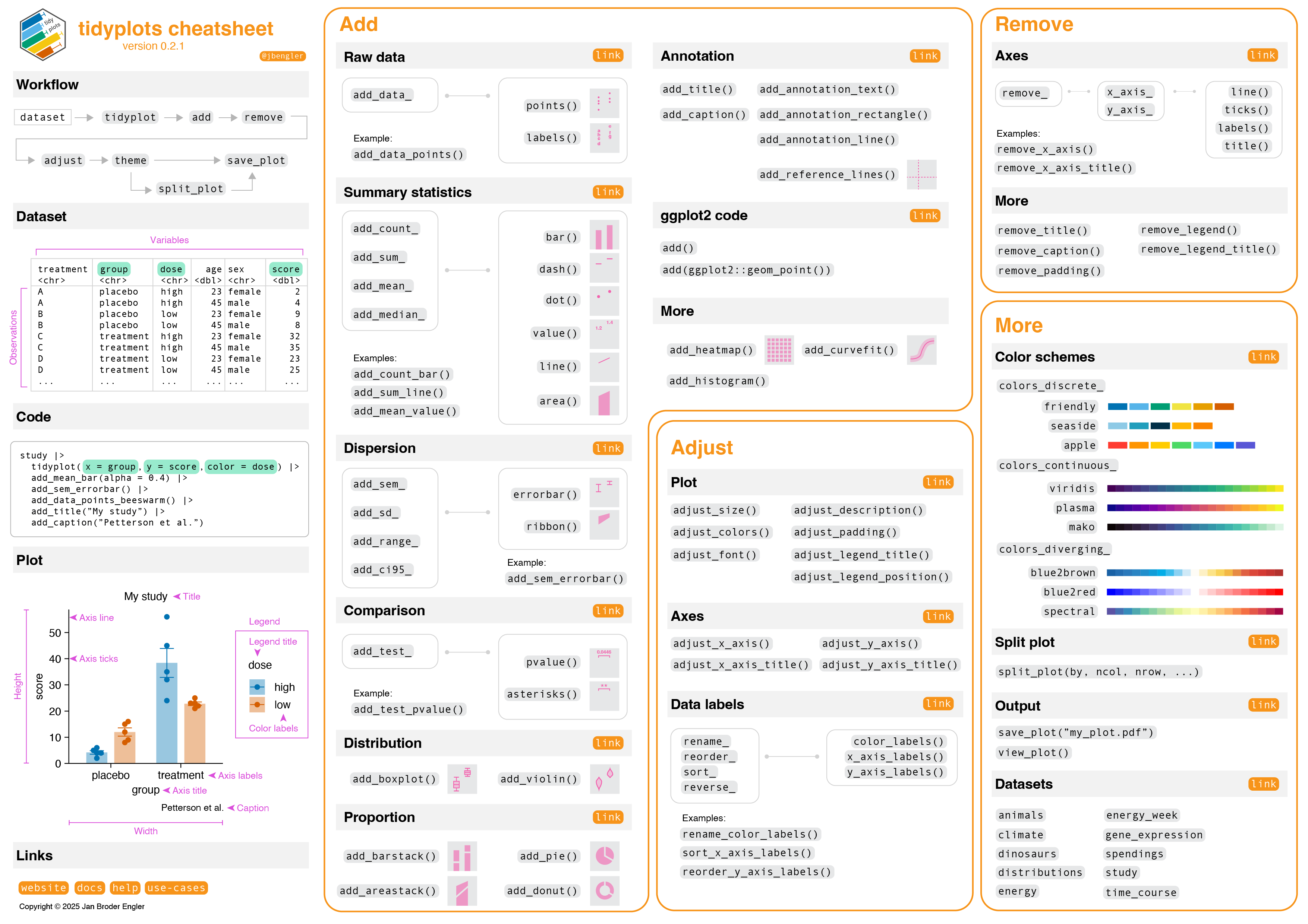
Cheatsheet

This cheatsheet gives a high level overview of available functions.

Usage

Here are some examples.

Also have a look at the getting started guide and the full documentation. For more example plots, check out the tidyplots use cases website.

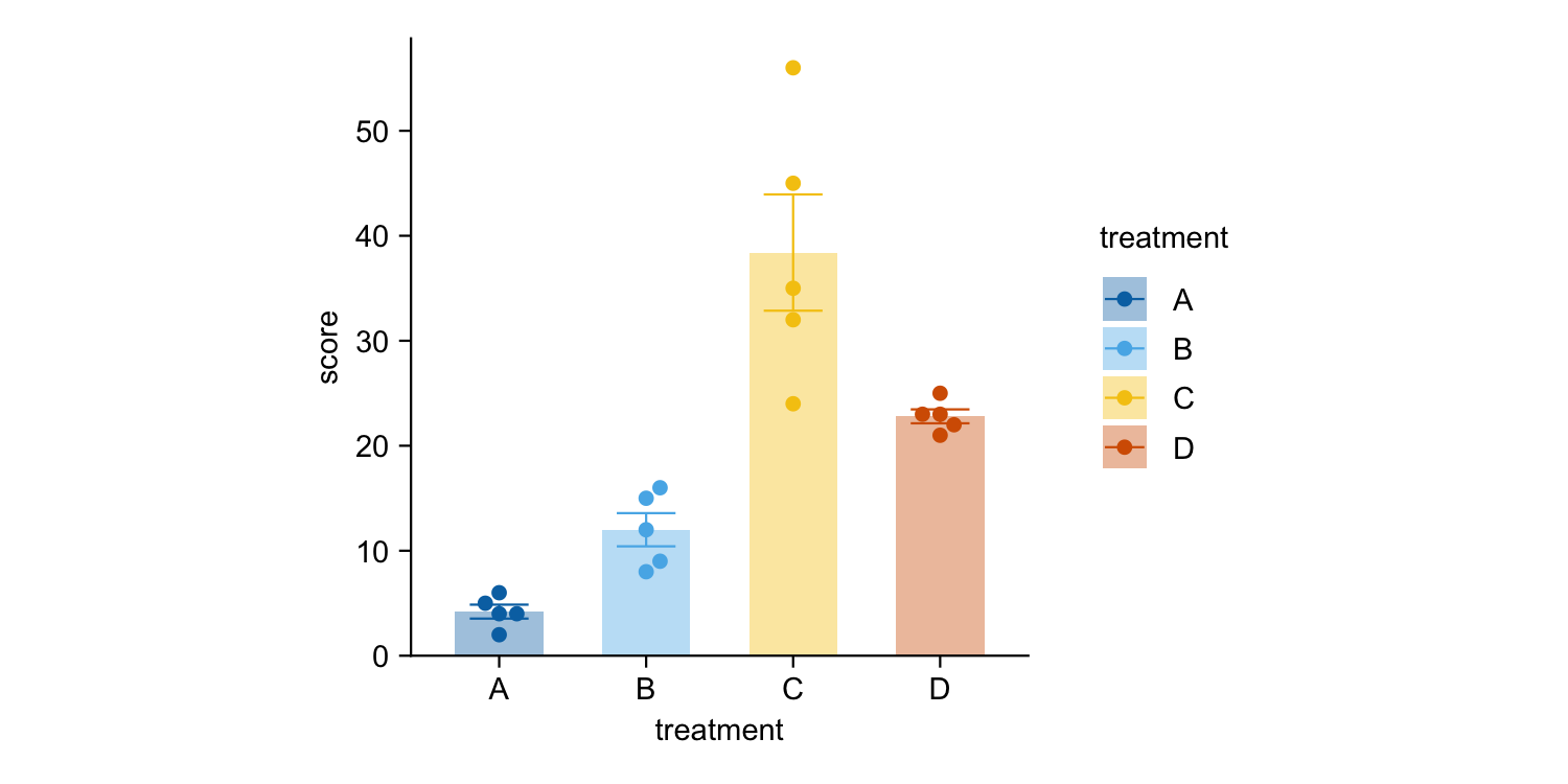
library(tidyplots)

study |> 
  tidyplot(x = treatment, y = score, color = treatment) |> 
  add_mean_bar(alpha = 0.4) |> 
  add_sem_errorbar() |> 
  add_data_points_beeswarm()

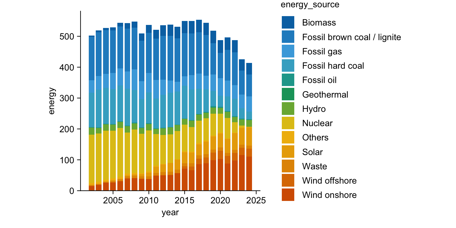
energy |> 
  tidyplot(x = year, y = energy, color = energy_source) |> 
  add_barstack_absolute()

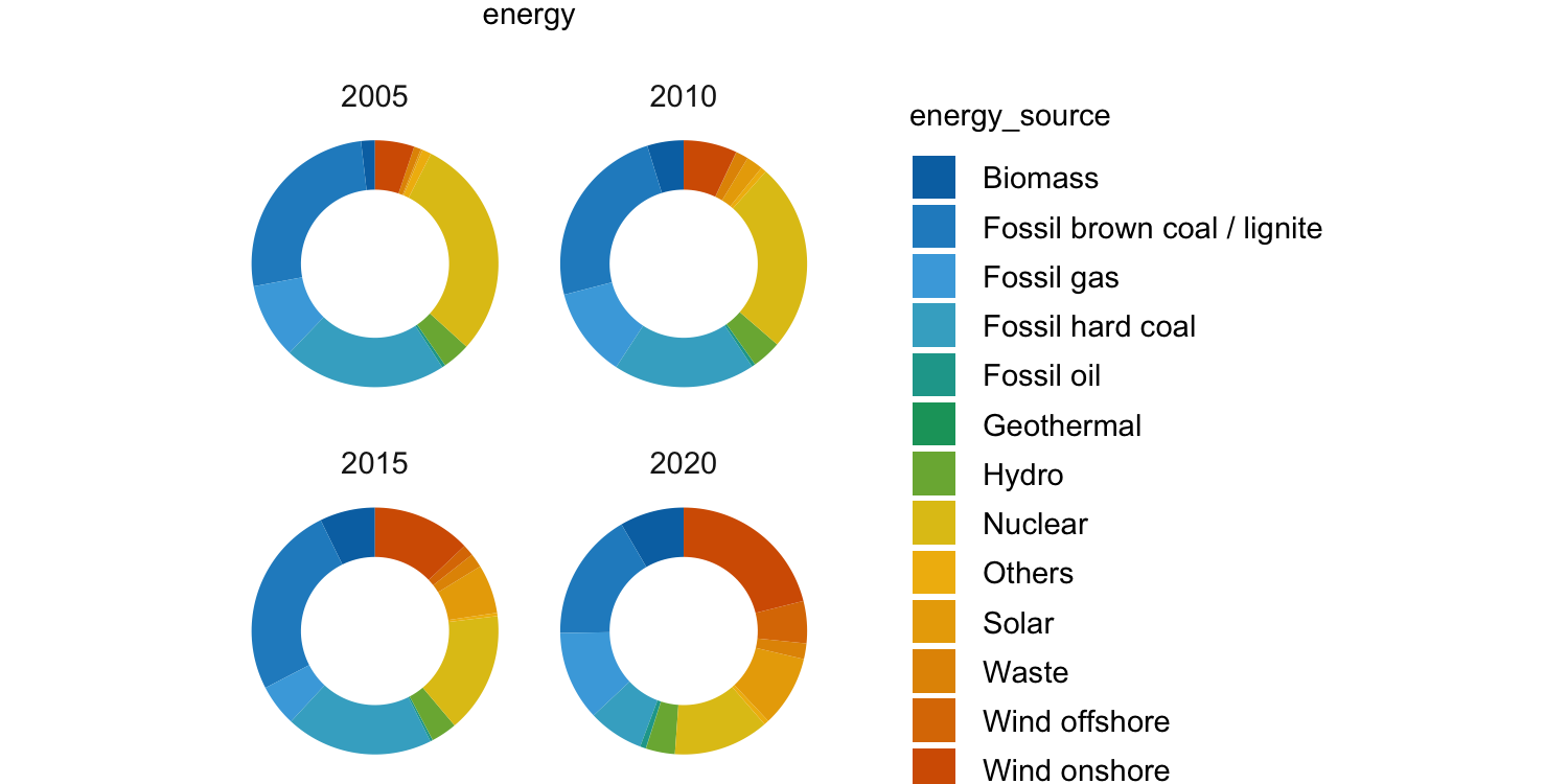
energy |> 
  dplyr::filter(year %in% c(2005, 2010, 2015, 2020)) |> 
  tidyplot(y = energy, color = energy_source) |> 
  add_donut() |> 
  adjust_size(width = 25, height = 25) |>
  split_plot(by = year)

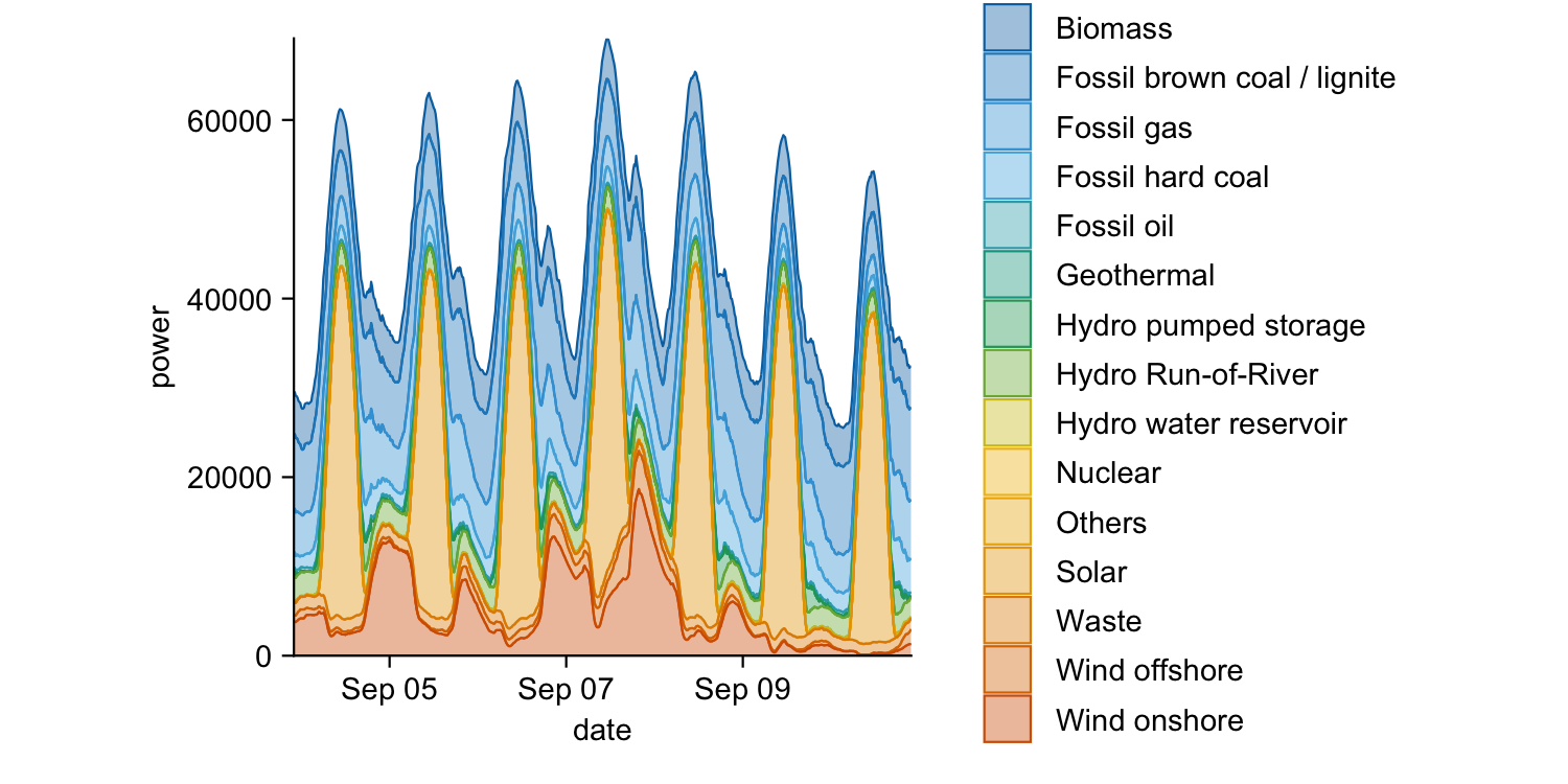
energy_week |> 
  tidyplot(x = date, y = power, color = energy_source) |> 
  add_areastack_absolute()

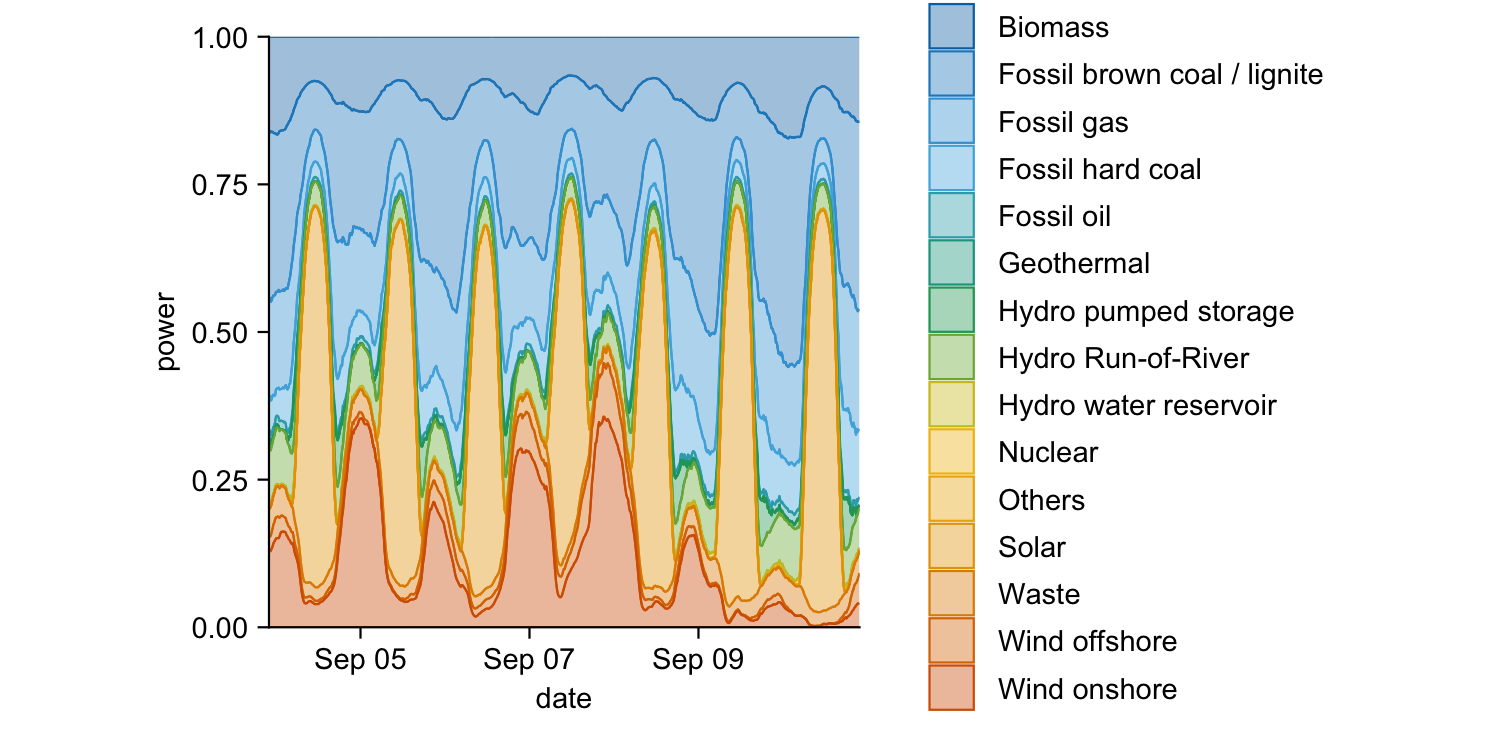
energy_week |> 
  tidyplot(x = date, y = power, color = energy_source) |> 
  add_areastack_relative()

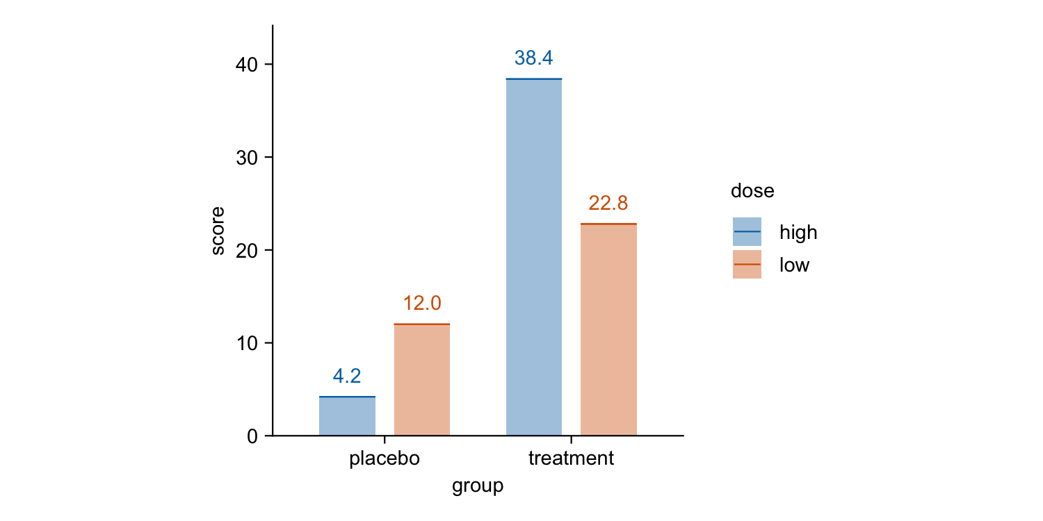
study |> 
  tidyplot(x = group, y = score, color = dose) |> 
  add_mean_bar(alpha = 0.4) |> 
  add_mean_dash() |> 
  add_mean_value()

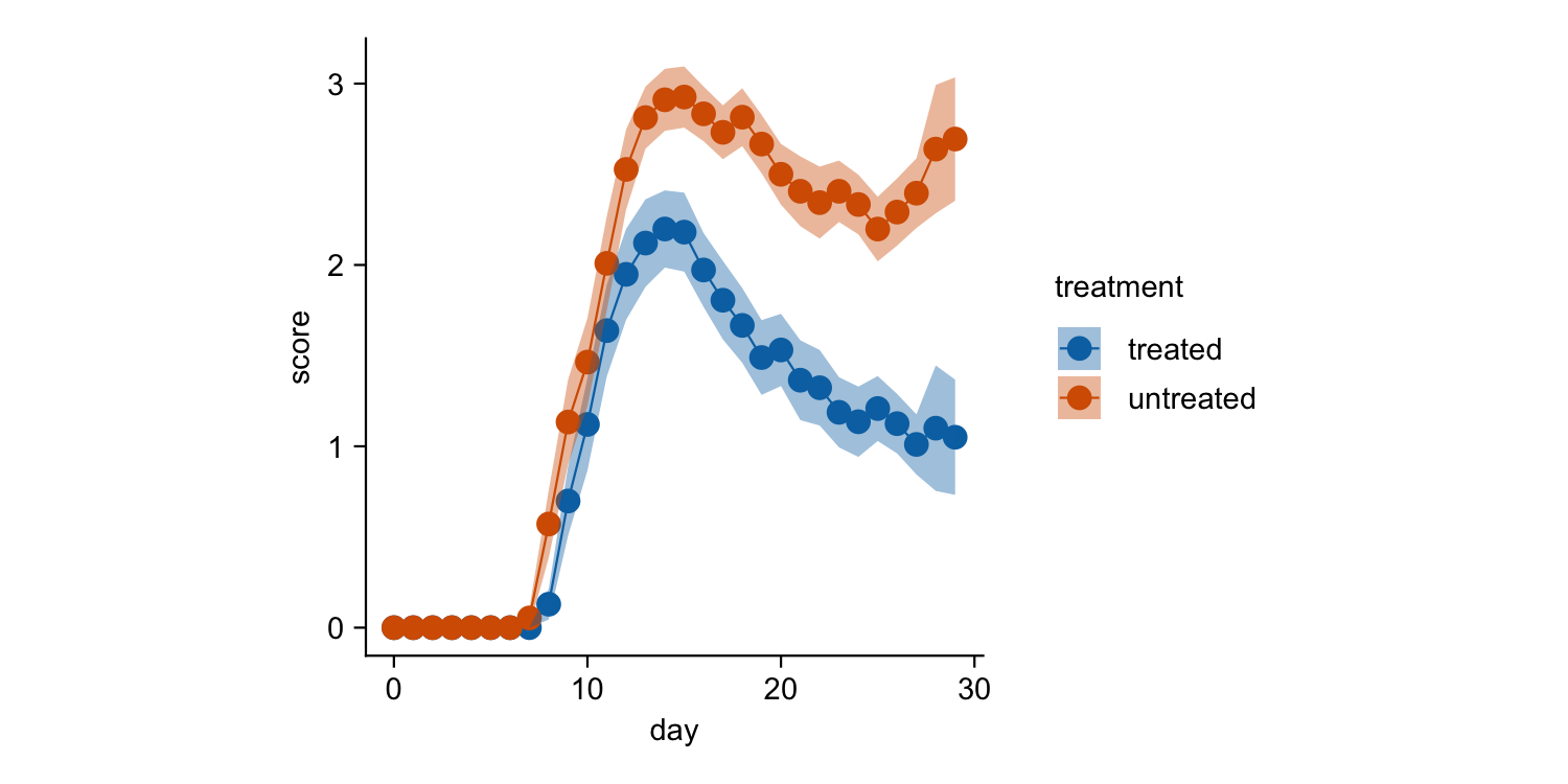
time_course |>
  tidyplot(x = day, y = score, color = treatment) |>
  add_mean_line() |>
  add_mean_dot() |>
  add_sem_ribbon()

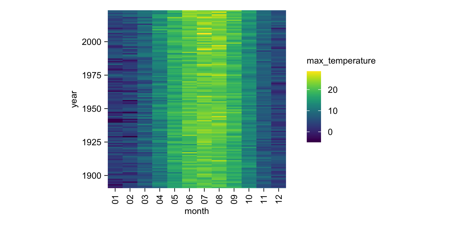
climate |>
  tidyplot(x = month, y = year, color = max_temperature) |>
  add_heatmap()

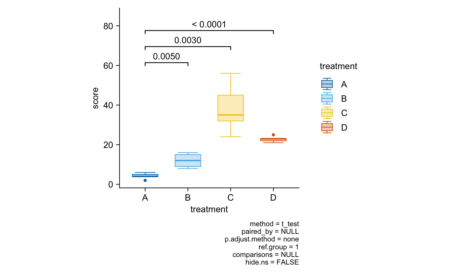
study |> 
  tidyplot(x = treatment, y = score, color = treatment) |> 
  add_boxplot() |> 
  add_test_pvalue(ref.group = 1)

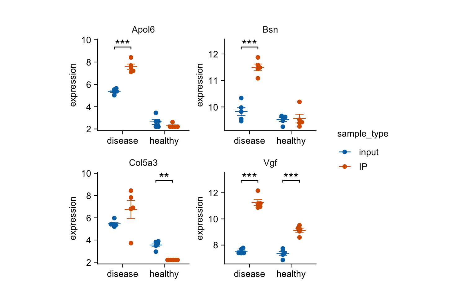
gene_expression |> 
  dplyr::filter(external_gene_name %in% c("Apol6", "Col5a3", "Vgf", "Bsn")) |> 
  tidyplot(x = condition, y = expression, color = sample_type) |> 
  add_mean_dash() |> 
  add_sem_errorbar() |> 
  add_data_points_beeswarm() |> 
  add_test_asterisks(hide_info = TRUE) |> 
  remove_x_axis_title() |> 
  adjust_size(width = 25, height = 25) |> 
  split_plot(by = external_gene_name)

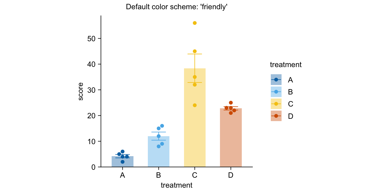
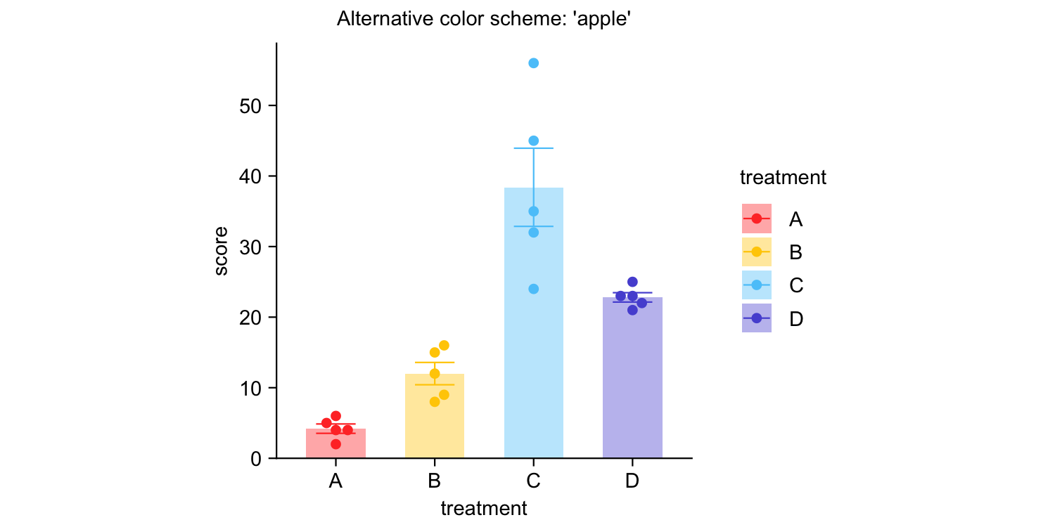
study |> 
  tidyplot(x = treatment, y = score, color = treatment) |> 
  add_mean_bar(alpha = 0.4) |> 
  add_sem_errorbar() |> 
  add_data_points_beeswarm() |> 
  view_plot(title = "Default color scheme: 'friendly'") |> 
  adjust_colors(colors_discrete_apple) |> 
  view_plot(title = "Alternative color scheme: 'apple'")

Documentation

• Package index
  Overview of all tidyplots functions

• Get started
  Getting started guide

• Visualizing data
  Article with examples for common data visualizations

• Advanced plotting
  Article about advanced plotting techniques and workflows

• Color schemes
  Article about the use of color schemes

Acknowledgements

I would like to thank Lars Binkle-Ladisch for our insightful discussions and for consistently challenging my decisions regarding the naming of functions and their arguments.

Many thanks to the R and tidyverse communities. tidyplots is built upon their software and coding paradigms, and it would not have been possible without their contributions.

tidyplots relies on several fantastic packages that handle all the heavy lifting behind the scenes. These include cli, dplyr, forcats, ggbeeswarm, ggplot2, ggpubr, ggrastr, ggrepel, glue, Hmisc, htmltools, lifecycle, purrr, rlang, scales, stringr, tidyr, and tidyselect.