
anseryuer/Local_LLM_Deployment_Guide_Chinese
anseryuer/Local_LLM_Deployment_Guide_Chinese has 58 GitHub stars and 4 forks. GitHot measured 0 stars in 24 hours, 0 in 7 days, and 0 in 15 days. Last checked 2026-11-16 03:16 UTC. Last push 2026-11-02.
Measured star growth
- in 24h
- 0
- in 7 days
- 0
- in 15 days
- 0
- in 1 month
- Update delayed
Net star changes over overlapping periods, not daily totals. Missing measurements are left blank. Stars measure attention, not software quality.
About
本地部署大语言模型的中文教学
AIREADME.en.md
OriginalRunning Large Language Models Locally: A Hands-On Guide
🌏 中文版: 本文的中文原版在 README.md。This English edition covers the same material; you only need to read one of them.
Last major revision: October 2026 Specific models, prices and commands change quickly, so I try hard to explain the why. That way, even after a model name goes out of date, you will still know how to judge things for yourself.
Hello everyone, Anser here!
You have probably used ChatGPT, Claude or DeepSeek and thought, "Wow, this is really cool." Then one day a thought pops up: could I run this on my own computer? No internet connection, no monthly subscription, no worrying that someone else can see what you talk about, and you can freely use it to build your own little tools.
Of course you can! This guide is written for you.
I got here by tinkering my way through it myself. I have used local models to build a multilingual translator and a small tool that summarizes long PDFs and online course videos, and I stepped into more pitfalls along the way than I can count. So I want to write down what I learned and save you some detours.
This guide walks you through it step by step: first we look at what your computer can do, then you get your first model running within ten minutes, and then, bit by bit, we work out what is actually happening behind the scenes.
- You don't need to know how to program, and you don't need to know machine learning. Every new term is explained the first time it appears.
- Later sections get very hardcore, for example multi-GPU parallelism, servers used by hundreds of people at once, and the FP4 number format. I have marked all of these, and you can safely skip them on a first read.
I may well make mistakes, and LLM hardware and software move absurdly fast. If you find anything wrong or out of date, please open an Issue or a PR. Thank you!
Support me: WeChat (click to see the QR code) · Buy me a coffee
Many thanks as well to the r/LocalLLaMA community. So many people generously share their hardware benchmarks, run settings and the pitfalls they hit, and I have learned an enormous amount from them.
Pick a route that fits you
This guide is long, but you do not need to read it from start to finish. Find the row that sounds most like you and follow the links in order:
| Where you are now | Suggested reading order |
|---|---|
| 🌱 I just want to get something running on my computer (most people start here!) | Step 0 → Part 1 → Part 2, and see Part 5 if you hit problems |
| 🧐 It already runs; I want to know why it is fast or slow and which model to switch to | Part 3 → Part 4 → Common misconceptions |
| 🛒 I am about to buy or upgrade hardware | Step 0 → Part 3 → Part 6, and Part 13 if you want to do the math |
| 🏢 I need to deploy a shared model for a team or company | Skim Part 2 and Part 3 first, then read Part 7 → Part 8 → Part 9 → Part 10 |
| 🔬 I'm just curious and want to understand how it works | After the beginner parts, read Part 11 and Part 12 |
Throughout the guide, three small markers tell you who a section is written for:
- 🌱 Beginner essential: read this the first time through.
- 🔧 Advanced: you can skip it on a first read and come back once you have things running and feel comfortable.
- 🔬 Deep dive: for the very curious. Skipping it does not affect your ability to use anything.
Contents
🌱 Beginner section
- Step 0: Take a look at your computer
- Part 1: Run your first model in ten minutes
- Part 2: What just happened?
- Part 3: Why is it sometimes fast and sometimes slow?
- Part 4: How to choose a model
- Part 5: What to do when something goes wrong
- Part 6: Should you upgrade your hardware?
🔧 Advanced section
- Part 7: More deployment tools
- Part 8: Serving many users: vLLM and high concurrency
- Part 9: Multiple GPUs, multiple machines and parallelism
- Part 10: Evaluating and comparing models seriously
🔬 Deep dives and doing the math
- Part 11: Precision and quantization
- Part 12: The math of speed limits and speculative decoding
- Part 13: Does running locally actually save money?
📚 Wrapping up
Step 0: Take a look at your computer
🌱 Beginner essential, about 10 minutes.
The question I get asked most is, "Can my computer run this?" Almost every computer can run a model of some size; the difference is how big and how fast. To answer the question, you first need to know what each piece of hardware does when a model runs, and how data moves between them.
A concrete machine as an example
Let's use a common high-end gaming PC as the example:
| Component | This machine | What it does when running an LLM | Key number |
|---|---|---|---|
| Storage | 2TB NVMe SSD (PCIe 4.0) | Holds the model file. Read only once, when the model loads | Sequential read about 7GB/s |
| System memory (RAM) | 32GB DDR5-6000, dual channel | A staging area during loading; when VRAM is too small, it holds the remaining model layers | Bandwidth about 96GB/s |
| CPU | AMD Ryzen 5 7600X, 6 cores | Splits text into tokens, drives the GPU, handles output; when VRAM is too small, computes the layers that live in RAM | FP32 peak about 1 TFLOPS |
| PCIe lanes | PCIe 4.0 x16 | Moves data between RAM and VRAM | About 32GB/s each direction |
| GPU | NVIDIA RTX 4090 | Runs the matrix multiplications, which are the vast majority of the model's computation | FP16 Tensor Core about 165 TFLOPS (FP32 accumulate, no sparsity) |
| Video memory (VRAM) | 24GB GDDR6X, soldered onto the card | Holds the model weights, the KV cache and intermediate results | Bandwidth 1,008GB/s |
Notice two comparisons first:
- Compute: the GPU does about 165 TFLOPS and the CPU about 1 TFLOPS, a difference of more than a hundred times.
- Bandwidth: VRAM is 1,008GB/s, system RAM is about 96GB/s, PCIe is about 32GB/s. The GPU reads VRAM about 10 times faster than the CPU reads RAM, and about 30 times faster than reading RAM over PCIe.
The GPU can only directly compute on data that is already in VRAM. So when running a model, we want the whole model to sit in VRAM.
Where the data lives and where the computing happens
Suppose we run an 8B-parameter model on this machine that is about 5GB after Q4 quantization (what "8B" and "Q4" mean is explained right below).
Loading (happens once): the model file is read from the SSD into system RAM, then copied over PCIe into VRAM. Reading 5GB from the SSD takes about 1 second, and copying it over PCIe about 0.2 seconds. Once loading finishes, the weights stay in VRAM.
You send a sentence: the CPU uses the tokenizer to split the text into a sequence of token IDs (a list of integers) and passes them to the GPU. Both the amount of data and the amount of computation in this step are tiny.
Generating each token:
- The GPU reads all ~5GB of weights out of VRAM and does one pass of matrix multiplication with the current token's data. The amount of computation is roughly
2 × number of parameters, about 16 GFLOPs; - At the same time it reads and writes the KV cache in VRAM (intermediate results for all previous tokens, covered in Part 3);
- It computes, for every token in the vocabulary, the probability that it comes next, and picks one;
- The chosen token is turned back into text and shown to you, and we go back to step 1.
Now let's work out how long step 1 takes:
Reading weights: 5GB ÷ 1,008GB/s ≈ 5 ms
Computing:       16 GFLOPs ÷ 165 TFLOPS ≈ 0.1 ms
Reading data is about 50 times slower than computing. The GPU spends most of its time waiting for data to arrive from VRAM, so the upper limit on generation speed is about 1 ÷ 5 ms ≈ 200 tokens/s. This situation, where you are limited by memory bandwidth, is called memory-bound.
If the same model sat entirely in system RAM and ran on the CPU, one pass over the weights would take 5GB ÷ 96GB/s ≈ 52 ms, for a limit of about 19 tokens/s.
Now an example that does not fit: a 70B model that is about 40GB after Q4 quantization. 24GB of VRAM can hold at most about 22GB of weights, and the remaining ~18GB sits in system RAM and is computed by the CPU. For every token generated:
GPU part: 22GB ÷ 1,008GB/s ≈ 22 ms
CPU part: 18GB ÷ 96GB/s    ≈ 188 ms
Total about 210 ms, a limit of under 5 tokens/s
Less than half of the weights live in RAM, yet they take 90% of the time. This is why "a model that doesn't fit in VRAM gets much slower."
That gives us a rule:
For a single user with one request processed at a time (batch size = 1): whether a model can run depends on whether the model and its KV cache fit in VRAM (or unified memory); how fast it runs depends on how many bytes must be read for each generated token, and how much memory bandwidth is available to read them.
This rule has preconditions. If many requests are processed together (a larger batch size), one read of the weights can serve several tokens at once, the amount of computation multiplies, and the bottleneck gradually shifts from bandwidth to compute. That is called compute-bound. The same happens when reading a very long input (prefill). Part 3 explains how to tell these cases apart.
Unified-memory machines
Apple M-series chips, AMD Strix Halo (Ryzen AI Max) and NVIDIA DGX Spark use unified memory: the CPU and GPU share the same pool of LPDDR memory. There is no separate VRAM and no copying over PCIe.
These machines have large capacity and medium bandwidth. For example:
| Machine | Max memory | Memory bandwidth |
|---|---|---|
| Apple M5 Max | 128GB | Up to 614GB/s |
| NVIDIA DGX Spark | 128GB | 273GB/s |
| AMD Strix Halo (Ryzen AI Max+ 395) | 128GB | 256GB/s |
The capacity is far larger than the RTX 4090's 24GB, and the bandwidth is between dual-channel DDR5 and the RTX 4090. So they can hold large models that a 4090 cannot, and their speed depends on how much data the model must read per token. Part 6 compares them in detail.
How to check your own hardware
Windows:
- Press
Ctrl + Shift + Escto open Task Manager and click "Performance". - Click "Memory" and look at total capacity and speed (for example 32GB, 6000 MT/s).
- Click "GPU" and look at the graphics card model and "Dedicated GPU memory": that is your VRAM. Many laptops have two GPUs (integrated and discrete); look at the NVIDIA or AMD one.
- With an NVIDIA card you can also press
Win + R, typecmd, press Enter, then runnvidia-smi. The output shows the model and VRAM size; for example24564MiBis about 24GB.
"Shared GPU memory" in Task Manager is not VRAM. It is system RAM that the GPU borrows over PCIe when VRAM runs out, at the speeds in the table above.
macOS: Apple menu → "About This Mac" shows the chip (for example M4 Pro) and memory (for example 48GB). Apple Silicon uses unified memory, and by default the system lets the GPU use roughly two-thirds to three-quarters of it, leaving the rest for the system and other programs.
Linux: nvidia-smi for the graphics card and VRAM, free -h for RAM.
Once you know the model, you can find the VRAM or memory bandwidth on the manufacturer's spec page. You will use that number throughout the rest of this guide.
Roughly how big a model can my computer run?
First, two terms that show up everywhere.
Parameter count (8B, 14B, 70B): each Transformer layer is made mainly of a few large matrices, for example 4096×4096 or 4096×14336. Every number in those matrices is called a parameter (also called a weight). "8B" means the model has about 8 billion such numbers in total (B = billion). During training, these numbers are adjusted over and over with huge amounts of text and gradient descent, so that the model predicts the next token more and more accurately; after training they are fixed, and at inference time the model just multiplies them with the input. More parameters usually means a more capable model, but also more memory and more data to read per token.
Quantization (Q4, Q8): original models usually store each parameter in BF16 format, 2 bytes each, so an 8B model is about 16GB. Quantization stores each parameter with fewer bits, for example 4 bits, plus an extra scale factor for each small group of parameters to restore approximate values. After Q4 quantization, each parameter averages about 4.5–5 bits, so an 8B model is about 5GB, roughly a third of the original size, usually with little quality loss. Local use almost always relies on quantized versions; details are in Part 2.
For common Q4 quantized versions, a rough estimate of weight size is parameter count (B) × 0.6 GB. Leaving room for context and the program itself gives the table below ("usable VRAM" means a discrete GPU's VRAM, or the part of unified memory the GPU can use):
| Usable VRAM/memory | Model size to try first | Matching Q4 weight size |
|---|---|---|
| No discrete GPU, 16GB RAM | 1B–4B, up to 8B | About 1–5GB, runs on the CPU |
| 6–8GB VRAM | 4B–8B | About 3–5GB |
| 12–16GB VRAM | 8B–14B | About 5–9GB |
| 24–32GB VRAM | 14B–32B | About 9–20GB |
| 64–128GB unified memory | 70B class, or 80B–120B class MoE models | About 40–75GB |
A real example: my old laptop had an AMD R5 7640U (a 28W low-power processor) + 32GB dual-channel DDR5-5600, no discrete GPU. The Q4 version of a 7B model is about 4GB, so the bandwidth estimate gives a limit of about 90GB/s ÷ 4GB ≈ 22 tokens/s, and I measured about 8 tokens/s. So even without a discrete GPU, you can chat normally with small models.
Next step
Now that you know your hardware, the next step is to run a model right away.
Part 1: Run your first model in ten minutes
🌱 Beginner essential. Run it first, theory later. Honestly, getting something running matters much more than researching whether to buy four GPUs.
To run a model you need an inference program (also called an inference framework or runtime). It reads the model file, puts the weights into VRAM or RAM, calls the GPU or CPU to compute, and provides a chat interface or an API. The two best options for beginners are:
| Program | Who it suits |
|---|---|
| LM Studio | You want a graphical interface and don't want to touch the command line. My top recommendation for your first time |
| Ollama | You are used to the command line, or you want other software to call the model |
Both are free, and both support Windows, macOS and Linux. Under the hood they are built on inference engines like llama.cpp (covered in Part 7). Let's walk through LM Studio first.
Running your first model with LM Studio
The interface updates often, so button names may not match exactly what I write, but the process is the same.
- Install: download the installer for your system from lmstudio.ai, install it and open it.
- Find a model: click the magnifying-glass icon on the left (Discover) and type a model name. For your first time, pick a 4B–8B model with Instruct or Chat in its name (these have been trained for conversation; see Part 2 for why), for example search
Qwen3 8B. If your VRAM is small, choose a smaller one using the table in Step 0. - Choose a file: the same model comes in several versions, with suffixes like
Q4_K_M,Q5_K_M,Q8_0. These are different levels of quantization: the smaller the number, the smaller and faster the file, and the slightly lower the quality. ChooseQ4_K_Mthe first time. LM Studio usually marks which versions fit entirely in your VRAM (something like "Full GPU Offload Possible"); prefer those. - Download: an 8B Q4 is about 5GB.
- Load: go back to the chat page, click "Select a model to load" at the top, and choose the model you just downloaded. Before loading, expand the settings and look at two options:
- Context Length: set it to
8192(8K) for now. The larger it is, the more VRAM the KV cache takes; the reason is in Part 3. - GPU Offload: slide it all the way up, which puts every layer on the GPU. If it won't go all the way, VRAM can't hold the model, some layers will stay in system RAM and be computed by the CPU, and speed will drop sharply, just like the 70B example in Step 0.
- Context Length: set it to
- Start chatting: type "Hi, tell me about yourself" and press Enter.
If you see text appearing word by word, the model is running on your computer.
The interface usually shows a speed such as 45 tok/sec, meaning 45 tokens generated per second. For reference:
- Over 20 per second: faster than reading speed, very smooth;
- 5–20: usable;
- Under 5: usually means part of the model didn't fit in VRAM; see Part 5.
You can also compare this number with the estimate in Step 0: measured speed usually reaches half to 80% of the "bandwidth ÷ model size" limit. If it is far below that, the GPU is most likely not being fully used.
Another option: Ollama
If you are comfortable with the command line, Ollama is more direct. Download and install it from ollama.com, then open a terminal (PowerShell or Command Prompt on Windows, Terminal on macOS) and type:
ollama run qwen3:8b
The first run downloads the model automatically; once it finishes you can chat right in the terminal. Type /bye to quit. Newer versions of Ollama also include a graphical chat window where you can pick a model and chat.
ollama list # list models you have downloaded
qwen3:8b is Ollama's model tag. Ollama picks a quantized version by default, usually around Q4; you can see exactly which on the model's page on the Ollama website.
Bonus: let other software use your model
Both LM Studio and Ollama can start a local API server. An API is an interface programs use to call each other: in a chat window you use the model directly, but when a note-taking app, an editor plugin or your own script wants to use the model, it calls the API through HTTP requests.
Lots of software supports an OpenAI-compatible API, meaning the request and response formats are the same as OpenAI's API. Change the server address in the software's settings from OpenAI to your own computer, and it will use the local model instead:
- LM Studio: turn on the local server on the Developer page; the default address is
http://localhost:1234/v1; - Ollama: runs at
http://localhost:11434by default once installed.
localhost means this computer. That is exactly how my translator and PDF summarizer are hooked up to local models.
Next step
Now that the model runs, the next part explains what the tokens, Q4_K_M and Context Length you just saw actually are.
If it didn't run, go straight to Part 5: What to do when something goes wrong.
Part 2: What just happened?
🌱 Beginner essential. This part explains the things you just saw in LM Studio or Ollama: tokens, how a model generates text, why you should choose the Instruct version, context length, and quantization.
If you want a systematic introduction to LLMs, I recommend two videos that need no programming or math background:
- Andrej Karpathy's Intro to Large Language Models: one hour that clearly explains how LLMs are trained and used;
- 3Blue1Brown's But what is a GPT?: animations of the computation inside a Transformer.
Tokens and the tokenizer
A token is the basic unit of a model's input and output. The model doesn't work on text directly; it works on a sequence of integers. The tokenizer uses a fixed vocabulary to cut text into pieces, then replaces each piece with its number in the vocabulary (its token ID). Vocabularies usually have over a hundred thousand entries; Qwen3's, for example, has about 150,000.
The pieces come in different lengths:
- In English, common words are usually one token, and uncommon long words are cut into several pieces;
- In Chinese, a common word or phrase may be one token, while an uncommon character may be a token on its own, or even be split into several;
- Emoji and rare symbols may be split into several tokens, each covering only a few bytes of the character's UTF-8 encoding.
The image below is OpenAI's Tokenizer demo page; each color is one token. The string of question marks at the end is one emoji split into several tokens, and a single one of those tokens can't be displayed as a complete character:
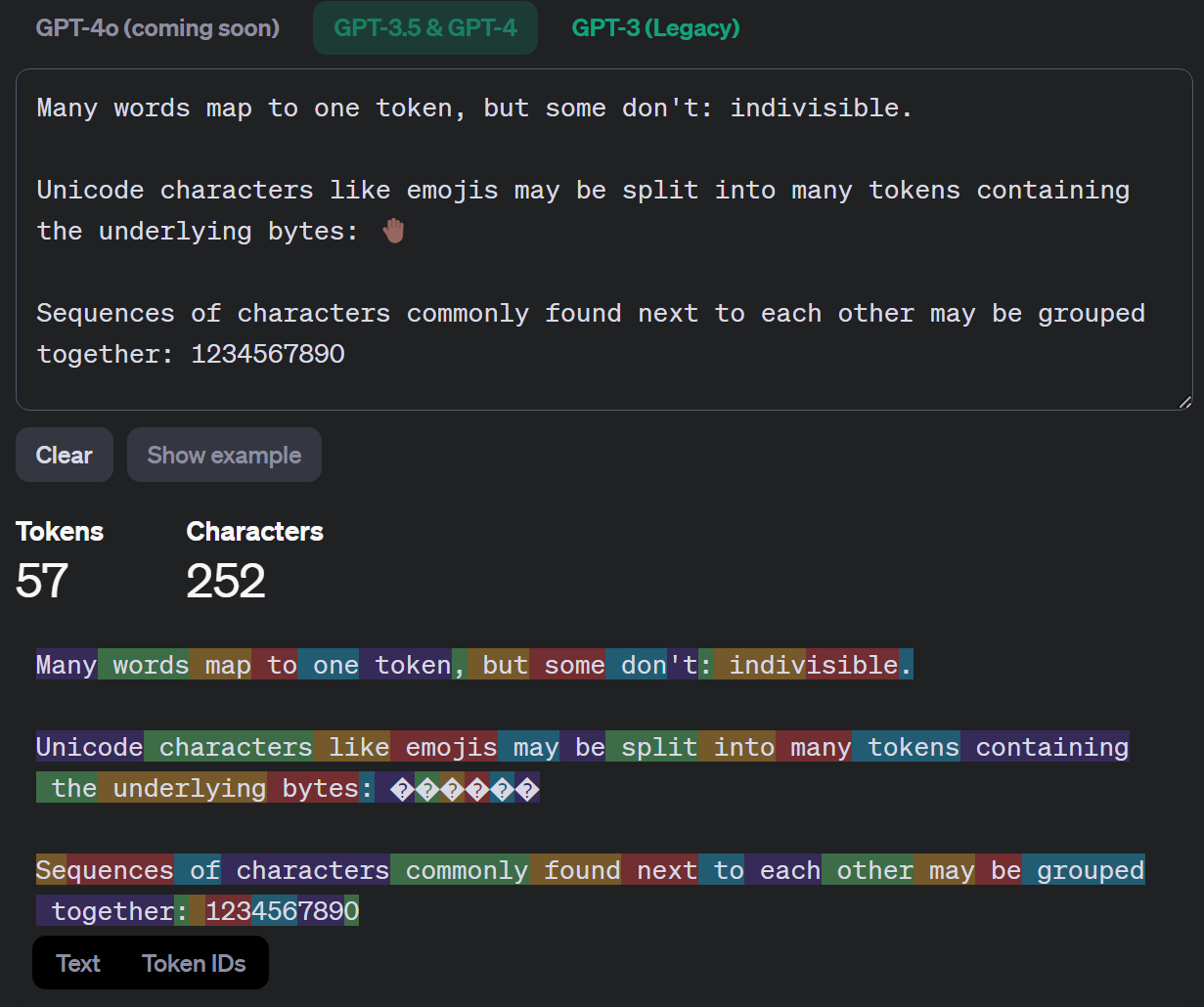
Different models have different vocabularies, so the same text produces a different number of tokens. If two models both show 50 tok/s, they don't necessarily produce the same number of words per second. Context length, API prices and generation speed are all counted in tokens, not words.
How a model generates text: one token at a time
Each run of the model (one forward pass) goes like this:
- Each token ID is turned into a vector (an embedding), for example 4096 numbers;
- These vectors pass through dozens of Transformer layers in turn. Each layer mainly does two things: attention (letting each token read information from all the tokens before it) and an MLP (a few more matrix multiplications on each token's vector);
- The last layer outputs a score for every token in the vocabulary, which is converted into a probability that "the next token is this one".
The program then picks one token from this probability distribution, appends it to the end of the input, and runs the model again to predict the one after that. This is called autoregressive generation. Generating 1000 tokens means running the model about 1000 times in sequence, and each run has to wait for the previous one to pick its result. That is why you see the text appear on screen piece by piece.
The rule for picking a token is controlled by a few sampling parameters:
- temperature: adjusts how flat the probability distribution is. Lower values favor the highest-probability token, giving stable output that tends to repeat itself; higher values make low-probability tokens more likely, giving more varied output that also makes more mistakes;
- top-p / top-k: only choose among the most probable tokens, filtering out very unlikely options.
The neural network architecture doing these calculations is the Transformer, from the legendary 2017 paper Attention Is All You Need. For years after it was proposed, the basic structure of mainstream LLMs hardly changed.
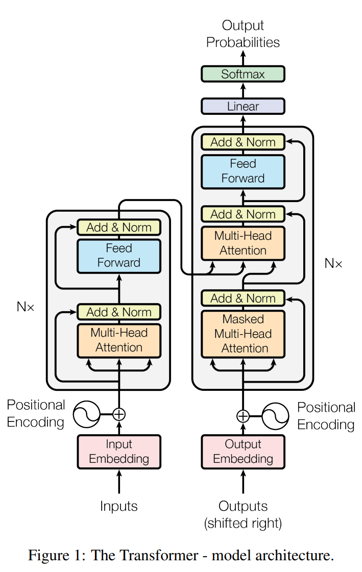
This figure is the original architecture from the paper. The left side is the encoder and the right side is the decoder, because the paper was designed for machine translation. Today's chat models are almost all decoder-only: they keep only the decoder structure on the right (minus the block that connects to the encoder) and stack it dozens of layers deep. Models with more parameters usually have more layers and bigger matrices in each layer.
Base models and instruct models
Training usually happens in two stages:
- Pre-training: the model is trained on huge amounts of text (web pages, books, code and so on) to predict the next token. The result is a base model. It has learned a great deal of knowledge, but it can only continue text. Give it "What is the capital of France?" and it may continue by writing a few similar quiz questions instead of answering.
- Post-training: training continues with conversation data, human preference feedback and reinforcement learning, so the model answers questions and follows instructions. The result is an instruct model (also called a chat model). ChatGPT was trained this way.
So when downloading, choose a version with Instruct or Chat in its name, or one clearly described as a chat model. Many models are now released as the chat version by default; one with Base in its name is usually not what you want.
Three related concepts:
- Chat template: the model's input is just a sequence of tokens. To tell "what the user said" apart from "what the assistant said", training wraps each turn of conversation in special tokens, such as
<|im_start|>user ... <|im_end|>. At inference time you must use exactly the same format as in training, or the model won't answer properly. Every model's template is different; LM Studio and Ollama usually read it from the model file and apply it automatically. With the wrong template, the model will ask and answer its own questions, output strange markers, or never stop. - System prompt: a piece of instruction placed at the very start of the conversation, such as "Answer only in English and keep answers short." Like a user message, it is just part of the input, but the model is trained to give it priority.
- Reasoning (thinking) models: before answering, these generate a thinking process (some interfaces fold it away) and then give the answer. They are usually more accurate on tasks like math and code, but they generate many more tokens, so they are slower. Many models and programs have a switch, and you can turn thinking off for everyday chat.
Context length
The model itself has no memory. In a multi-turn conversation, the program sends the entire chat history plus your new question to the model as input every time. The maximum number of tokens the model can handle at once is its context length, for example 8K, 32K or 128K, and it is decided during training.
Once the chat history exceeds the context length, the program has to drop or compress the earliest content, and the model can no longer see what was said at the beginning.
A bigger context is not always better:
- It uses memory. The model keeps an intermediate result (the KV cache) for every token in the context. It grows linearly with context length, and with a long context it can be bigger than the model itself. That is why I suggest starting with 8K in LM Studio. Part 3 does the actual calculation.
- Fitting it in doesn't mean using it well. A model that claims 128K support won't necessarily still find and use every detail accurately in a 128K input.
Vendors often test the second point with a needle-in-a-haystack test: insert one sentence somewhere in a long document, then ask the model about that sentence. The image below is the result Anthropic published when it released Claude 3 Opus: the horizontal axis is context length, the vertical axis is where the sentence sits in the document, and greener means more accurate retrieval.
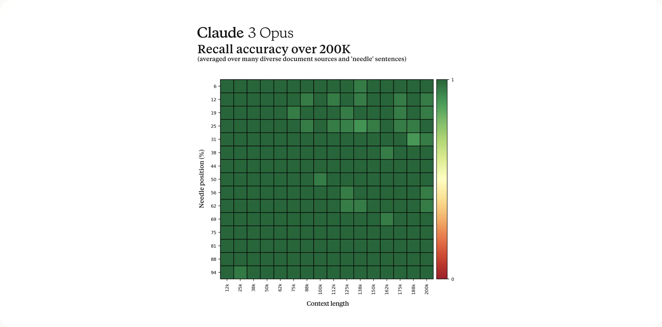
Top models now score close to perfect on this test, but it only checks "can it find one sentence". Real tasks usually require understanding and synthesizing the whole document, which is much harder, and small local models are generally much weaker on long context than top models. My advice: 8K is enough for everyday chat; for long documents, use 16K–32K and test with your own documents whether the model actually understood them.
Quantization: what Q4_K_M actually means
Step 0 said that quantization stores each parameter with fewer bits. Here is how to read the suffix in a GGUF file name:
- Q: quantized;
- 4: about 4 bits per parameter (a bit more on average once scale factors and other auxiliary data are added);
- K: k-quant, a llama.cpp quantization method that computes scale factors separately for small blocks, with less error than earlier methods;
- M: medium. Each level usually comes in S (small), M and L (large); larger keeps more precision.
How much quality does quantization cost? The chart below comes from the tests run when llama.cpp introduced k-quants:
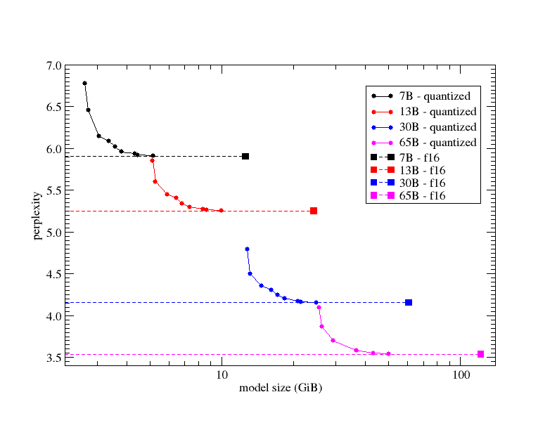
How to read it:
- The horizontal axis is model file size, and the vertical axis is perplexity. It measures how accurately the model predicts each next token in a test text; lower is better. It correlates with real task performance but is not the same thing;
- Each color is one model size, and the dashed line is the unquantized (f16) perplexity;
- Further left on the same curve means more aggressive quantization and a smaller file.
From the chart you can see:
- At the middle quantization levels, the curve almost touches the dashed line, so quality loss is small;
- At the leftmost Q2 level, the curve bends up sharply and quality drops a lot;
- In this set of tests, a quantized large model is still better than an unquantized small one; for example 13B at Q4 beats 7B at f16.
This chart was measured on LLaMA models in 2023, so the specific numbers are out of date, but the pattern basically still holds. My recommendations:
- Choose
Q4_K_Mby default: the best balance of size and quality; - If you have VRAM to spare, choose
Q5_K_MorQ6_K;Q8_0is nearly lossless but almost twice the size of Q4; - Only consider Q3 when nothing else fits; Q2 is the last resort; Q1 is basically unusable;
- The smaller the model, the more sensitive it is to quantization; math, code and long-context tasks are also more easily affected.
"A large model at Q2 always beats a small model at Q5" is not guaranteed. Test each on your own tasks.
You will see other formats on download pages too:
- GGUF: the model file format defined by llama.cpp, used by both LM Studio and Ollama. The Q4_K_M above is a GGUF quantization level. For personal local use, just look for GGUF.
- safetensors: the most common format for original models, usually unquantized and large, mainly used by server programs like vLLM.
- GPTQ, AWQ, FP8, NVFP4, MLX and others: other quantization methods or formats aimed at specific programs or hardware (MLX is for Apple chips only). See Part 11.
Next step
You now know how a model generates tokens one at a time, why to choose the Instruct version, and what context and quantization are. The next part expands the estimation method from Step 0: how to estimate speed for different hardware and different models, and when you are limited by bandwidth versus compute.
Part 3: Why is it sometimes fast and sometimes slow?
🌱 Beginner essential. Only multiplication and division are needed. After this part, you will be able to estimate "roughly how fast this model runs on this machine" yourself, and understand most hardware reviews.
Step 0 worked through one calculation on an RTX 4090: generating one token took 5 ms to read the weights and only 0.1 ms to compute. This part generalizes that method to different hardware and different ways of using it.
Four hardware metrics
Capacity (GB): whether VRAM or RAM can hold the model weights, the KV cache and the other data needed at runtime. If it can't, your only options are a smaller model, lower quantization, a shorter context, or putting part of it in slower memory. No amount of compute solves a capacity problem.
Memory bandwidth (GB/s): how much data can be read from VRAM or RAM per second. With one user and one request at a time, it mostly determines generation speed.
Compute (FLOPS): how many floating-point operations can be done per second. It becomes important when processing long inputs, serving many requests at once, and training. GPU spec sheets usually list the Tensor Core peak at some precision (FP16, FP8, FP4).
Interconnect bandwidth: how fast data moves between GPUs and between machines, for example PCIe, NVLink or the network. You don't need to think about it with a single card; with several cards it can become the bottleneck. See Part 9.
Estimating single-user generation speed
With one user and one request at a time (batch size = 1), generating each token requires reading almost all the weights from memory once, so:
Generation speed limit (tokens/s) ≈ memory bandwidth (GB/s) ÷ weights read per token (GB)
For an ordinary (non-MoE) model, "weights read per token" is just the model file size. Taking an 8B model that is about 5GB after Q4 quantization:
| Device | Memory bandwidth | Limit |
|---|---|---|
| Dual-channel DDR5-5600 RAM, CPU compute | About 90GB/s | About 18 tokens/s |
| AMD Strix Halo (Ryzen AI Max+ 395) | 256GB/s | About 51 tokens/s |
| RTX 4060 Ti 16GB | 288GB/s | About 58 tokens/s |
| Apple M5 Max (top configuration) | 614GB/s | About 123 tokens/s |
| RTX 3090 | 936GB/s | About 187 tokens/s |
| RTX 4090 | 1,008GB/s | About 202 tokens/s |
| RTX 5090 | 1,792GB/s | About 358 tokens/s |
These are upper limits. In practice the program also reads the KV cache, converts quantized data back into the format used for computation, and launches GPU work, and hardware rarely sustains its rated bandwidth, so measured speed is usually 50% to 80% of the limit. The formula is best used for comparison: for the same model, doubling the bandwidth roughly doubles the speed; halving the model size also roughly doubles it.
It directly explains a few common observations:
- Q4 is faster than the original BF16: the data read per token drops from 16GB to about 5GB;
- Speed collapses when some layers don't fit in VRAM: those weights must be read from system RAM at about 90GB/s. In the 70B example in Step 0, less than half the weights took 90% of the time;
- A Mac runs models faster than the CPU of a similarly priced PC: the unified memory bandwidth of M-series chips is several times that of ordinary dual-channel RAM.
Memory-bound and compute-bound
Whether a computation is limited by bandwidth or by compute depends on how many operations are done per byte read. This is called arithmetic intensity.
Taking the RTX 4090 as an example, its ratio of compute to bandwidth is about:
165 TFLOPS ÷ 1,008GB/s ≈ 164 FLOPs/byte
This means: for every byte read, at least about 164 operations must be done to keep the compute fully busy. Below that, the GPU is waiting for data (memory-bound); above it, bandwidth is to spare and the GPU is busy computing (compute-bound).
Q4 weights average about 0.6 bytes per parameter, and each parameter does 2 operations (one multiply, one add) per token:
- Processing 1 token at a time (one user generating token by token): 2 operations per 0.6 bytes read, about 3 FLOPs/byte, far below 164, so it is memory-bound;
- Processing N tokens at a time: one read of the weights is shared by N tokens, so arithmetic intensity is about
3 × N. When N reaches about 50, it starts to approach the 4090's compute limit and becomes compute-bound.
When do you process many tokens at once? In two cases:
- Processing the input (prefill): the several thousand tokens you send can be computed together;
- Serving many requests at once (batching): many users' requests are combined, and at each step every request generates one token.
In both cases, compute becomes important.
🔬 A more precise calculation (including a full numerical example on the H200) is in Part 12.
Prefill and decode
A request has two phases:
Prefill: the model processes the entire input at once, including the system prompt, chat history, documents and question, and produces the first token. All tokens in the input can be computed together, so this is compute-bound. For example, processing a 2,000-token input with an 8B model on an RTX 4090 takes about 2,000 × 16 GFLOPs = 32 TFLOPs of computation, at least about 0.2 seconds at 165 TFLOPS; attention computation comes on top of that, and the longer the input, the faster the attention part grows.
Decode: after that, each step generates one token, and each step reads all the weights once, so it is memory-bound (for a single user).
That is why after you paste in a long article, you wait a while before the first word appears, and once words start appearing the speed is fairly steady. The time from sending the request to seeing the first token is called TTFT (Time To First Token) and is mainly determined by prefill; the tokens/s after that is mainly determined by decode.
So when comparing hardware, you can't look only at compute or only at bandwidth: compute determines how fast long inputs are processed, and bandwidth determines how fast a single user's output is generated.
KV cache: why you don't recompute from scratch every time
Attention in a Transformer lets each token read information from all the tokens before it. Concretely, each layer computes two vectors for each token, the Key (K) and the Value (V); a new token compares its own vector with the K of all previous tokens, then takes a weighted combination of their V according to the comparison results.
In the causal Transformer used by chat models, each token can only see the tokens before it. Once token 100 appears, the K and V of tokens 1–99 don't change. So when generating token 101, the K and V of the first 100 tokens can be reused directly without recomputing. The program keeps them in VRAM, and this block of data is called the KV cache.
- Without a KV cache: generating token
tmeans recomputing the K and V of allt-1previous tokens in every layer, getting slower and slower; - With a KV cache: each token's K and V are computed only once, when it first enters the model, and then read straight from VRAM.
The cost is VRAM, proportional to the context length and the number of conversations running at the same time:
KV cache bytes ≈ 2 × layers × KV heads × head dimension
                 × bytes per element × cached tokens × concurrent sequences
The leading 2 is for the two copies, K and V. The number of layers, KV heads and the head dimension are listed in the model's config.json.
For example, a model with 32 layers, 8 KV heads and a head dimension of 128, storing the KV cache in 16 bits (2 bytes), needs this for one 32K context:
2 × 32 × 8 × 128 × 2 bytes × 32768 ≈ 4 GiB
A 128K context is about 16GiB; eight such conversations at once multiplies that by 8.
So after you put a 20GB model on a 24GB card, the remaining space isn't necessarily enough for a long context: the KV cache for a single 32K context alone takes about 4GiB, before other runtime overhead. That is also why Part 1 suggests starting with 8K.
The KV cache is also read during decode, so with a very long context, each token has to read a big chunk of KV cache in addition to the weights, and speed drops too.
🔧 Newer models use structures like GQA, MQA and MLA to reduce how much K/V data each token needs to store. Some programs can also quantize the KV cache to 8 or even 4 bits to save more VRAM, but this may hurt long-context accuracy; and if the program has no matching low-precision compute code, it may only save capacity without speeding anything up.
How much memory does a model actually take?
Counting only the weights:
Model weights in GB ≈ parameter count (B) × bits per parameter ÷ 8
For an 8B model:
| Precision | Raw weight size |
|---|---|
| FP32 (32-bit) | 32GB |
| FP16/BF16 (16-bit, common for original models) | 16GB |
| FP8/INT8 (8-bit) | 8GB |
| 4-bit | 4GB |
Actual files are a bit larger, because they also store scale factors and other auxiliary data, and some layers aren't quantized. For GGUF Q4_K_M you can estimate 4.5–5 bits per parameter; once downloaded, go by the actual file size.
Total usage at runtime is:
Model weights + KV cache + intermediate results (activations) + inference program overhead + system and other programs
So you can't use all 24GB of VRAM for weights. Leave at least 10%–20% in general; with long contexts or many concurrent users, work out the exact number with the KV cache formula above. Also, games, browser videos and other AI software running at the same time take up VRAM too.
Being able to run inference on a model doesn't mean you can train it. Besides the weights, training has to store gradients, optimizer states and more. With common mixed-precision Adam training, each parameter can take around 16 bytes, 8 times as much as BF16 inference, not counting activations. Methods like LoRA/QLoRA greatly reduce the memory needed for training.
MoE: huge total parameters, small active parameters
You will often see names like 80B-A3B or 235B-A22B. These are MoE (Mixture of Experts) models.
In an ordinary model (also called a dense model), each layer's MLP uses all of its parameters for every token. MoE splits the MLP into many smaller "expert" networks, and each layer also has a router that picks a few of them for each token (for example 8 out of 128) to take part in the computation; the other experts skip that step.
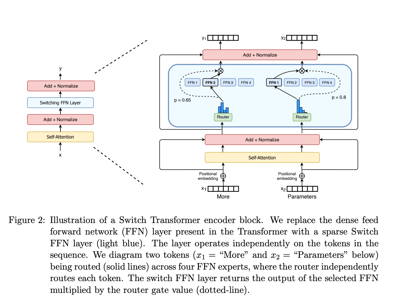
So an MoE model has two parameter numbers:
- Total parameters (the 80B in the name): all experts added together, which determines how much memory it takes;
- Active parameters (the A3B in the name): the parameters actually used for each token, which determines roughly how much data is read and how much computation is done per token.
For example, Qwen3-Next-80B-A3B has about 80B total parameters with 3B active per token; Qwen3.8-Flash-Next, released in August 2026, has 125B main-model parameters with 6B active per token, plus 51B of N-gram embeddings. They need the memory capacity of a large model, but their single-user generation speed is close to a much smaller dense model.
Let's do the math: an 80B model at 4.5 bits per parameter has about 45GB of weights and needs more than 64GB of usable memory. With 3B parameters active per token, the weights read per token are about 3B × 4.5 ÷ 8 ≈ 1.69GB. On a 256GB/s Strix Halo, the limit is about 256 ÷ 1.69 ≈ 151 tokens/s. In practice it also reads attention layers, shared experts, the KV cache and so on, so it will be noticeably lower than this, but a 45GB dense model in the same memory has a limit of only 256 ÷ 45 ≈ 6 tokens/s. This is why unified-memory machines with large capacity and medium bandwidth are especially well suited to MoE.
But MoE is not free of bandwidth limits:
- Non-expert parts such as attention and shared experts are used for every token;
- Which experts each token uses is decided dynamically, so memory access isn't contiguous and real efficiency suffers;
- When many requests are processed together, different tokens choose different experts, and in one step most experts may have to be read;
- When experts are spread across several cards, data has to travel back and forth between cards;
- If expert weights sit in system RAM, they have to cross PCIe to the card every time (PCIe 4.0 x16 is about 32GB/s), and speed is limited by PCIe.
One user versus many users
Most of the estimates above are for one user. If a team of dozens or hundreds of people shares one model, things are different: the server combines many requests, and one read of the weights can generate one token for each of dozens of requests at the same time. Following the memory-bound / compute-bound analysis above, the server's total tokens per second will be much higher, but the speed each user gets will drop and queueing time will grow. Part 8 covers this in detail.
Summary
- Whether it can run: look at capacity; weights + KV cache + other overhead must fit;
- Single-user (batch size = 1) generation speed: look at bandwidth; the limit ≈ bandwidth ÷ weights read per token;
- Long inputs (prefill) and many users (large batches): compute starts to become the limit;
- MoE: total parameters determine memory use, and active parameters determine roughly how fast it runs for a single user.
The next part uses these methods to choose a model.
Part 4: How to choose a model
🌱 Beginner essential.
No model is best at every task. The order for choosing is: first filter out what your hardware can't run, then compare the rest on your own tasks.
Step one: filter out what you can't run
However strong a model is on a leaderboard, it is useless if it won't run on your computer. So the first step is always to filter with the method from Part 3:
- Does it fit? The model file + KV cache + other overhead must fit in your VRAM or unified memory;
- Is it fast enough? Estimate the speed limit with "bandwidth ÷ model size", knock some off, and see whether you can live with it;
- Does your program support it? Very new model architectures may not run until LM Studio, Ollama or llama.cpp has been updated.
An example: with a 24GB card, leave 6GB for the KV cache, the inference program and the operating system's desktop, and about 18GB is left for the model. A 27B model at 4.5 bits per parameter is about 15.2GB, which fits; a 70B model needs about 39.4GB for the weights alone, so it is out. If the card has about 1,000GB/s of bandwidth and the 27B model's actual file is 17GB, the speed limit is about 1,000 ÷ 17 ≈ 59 tokens/s. Measured speed will be somewhat lower, but that is already very comfortable for chat.
Also, you don't have to use the biggest model you can run; good enough is good enough. If an 8B model can do your task, it will be three to four times faster than a 32B model and leave more VRAM for long context.
Some models to try right now
This section was written in August 2026. Models get a new round of releases roughly every three months, and each generation is stronger than the last at the same size. When you read this, search LM Studio or Hugging Face for the latest version of the same family at the same size.
Following the VRAM tiers from Step 0, here are some directions to try first:
| Usable VRAM/memory | Try this size first | Examples |
|---|---|---|
| Around 8GB | 4B–8B | Qwen3-8B (the one used in Part 1) |
| 12–16GB | 8B–14B | Qwen3-14B, Gemma 3 12B |
| 24–32GB | 27B–32B | Qwen3.8-27B, Gemma 3 27B |
| 64–128GB unified memory | Large MoE | Qwen3-Next-80B-A3B, Qwen3.8-Flash-Next |
If you work in Chinese, Chinese model families such as Qwen, DeepSeek, GLM and Kimi are generally better at it; families like Gemma, Llama and Mistral each have their own strengths too. Keep two things in mind when choosing:
- Different models are optimized in very different directions. Some are good at writing code, some at multiple languages, some at tool calling. The best approach is to take a few questions you ask often and try them on each model in turn.
- Choose the chat version (instruct/chat), not the base version. The reason is in Part 2.
Where to download: Hugging Face
Hugging Face is a site that hosts model weights and datasets, and almost every open model is released there. LM Studio's search feature searches Hugging Face, so with LM Studio you don't need to download from the site yourself.
If you want to look on the site yourself, a model page usually has:
- Model card: describes what the model can do, how long its context is, what its license is, and the recommended settings;
- Files: the model files themselves.
Original models are usually in safetensors format and very large. To run with LM Studio, Ollama or llama.cpp, search for "model name + GGUF". Many official teams publish their own GGUF versions (for example Qwen/Qwen3-8B-GGUF), and there are also people and teams in the community who specialize in quantization (for example unsloth and bartowski) and turn popular models into all kinds of quantization levels. Just find the file with Q4_K_M in the file list.
Try before you download
Models are often several GB to tens of GB, so you can try them online before downloading:
- Many models have an online version you can chat with directly on the official website or the Hugging Face page (on Hugging Face these are called Spaces);
- LMArena: shows two anonymous models' answers to the same question, lets users pick the better one, and aggregates lots of votes into a leaderboard. You can ask questions there to compare models directly, or look at its leaderboards split by language, code, long text and other categories.
Remember, though: a high leaderboard score doesn't mean it suits your task best. Human preferences can be specifically "pandered to"; for example, longer answers with nicer formatting tend to get picked more often. Leaderboards are good for narrowing things down, but in the end you have to try for yourself.
🔧 Want to compare models seriously, for example to choose a model for your company or build your own test set? See Part 10.
Don't forget to check the license!
"Downloadable" doesn't mean "use however you like". If you are just playing with it yourself or doing research, you are generally fine; but if you want to make money with it (commercial use), read the license carefully.
- Licenses like Apache-2.0 and MIT generally allow commercial use, but please read the actual text;
- Some models use custom licenses that may limit the number of users, require attribution, forbid using their outputs to train other models, or restrict regions and uses;
- Anything with NC (Non-Commercial) in it, like CC-BY-NC, forbids commercial use. Use it in a paid app and you may well get a letter from a lawyer.
The license is on the model page; read the original text for the version you downloaded. Before real commercial use, it is best to have someone who knows the law check it.
Next step
Once you have chosen a model and it runs, see the next part if you run into problems; if everything goes smoothly, you can skip straight to Part 6, or go to Common misconceptions to check you haven't fallen into a trap.
Part 5: What to do when something goes wrong
🌱 Beginner essential. Below are the most common kinds of problems and the order to troubleshoot them in.
The model fails to load, or says it is out of memory
The model plus its context doesn't fit. Try these in order:
- Reduce the context length, for example from 32K down to 8K;
- Close programs that use VRAM, such as games, videos in the browser, and other AI software;
- Switch to a smaller quantization level, for example from Q5_K_M to Q4_K_M;
- Lower GPU Offload (also called the number of GPU layers): leave some layers in ordinary RAM for the CPU to compute. It will run, but slower;
- Switch to a smaller model.
It is extremely slow (only a few tokens per second)
The most common cause is that the model isn't entirely in VRAM, and some layers are in system RAM being computed by the CPU (see Step 0 for why):
- In LM Studio, check whether GPU Offload is at the maximum and whether there is a message about "partial offload";
- Open Task Manager's "Performance → GPU" and watch, while chatting, whether "Dedicated GPU memory" is close to full and whether the GPU is busy;
- If "Shared GPU memory" usage is high, VRAM isn't enough and the GPU is borrowing system RAM over PCIe;
- On a laptop, plug in the power and make sure you are using the discrete GPU, not the integrated one;
- An old graphics driver can also stop the GPU from being used; update the driver.
If the model really is bigger than your VRAM, slowness is normal. Use the steps above to switch to a smaller model or quantization level.
It takes a long time before the first word appears
- The input is too long: the model has to process the entire input (prefill) before it can generate the first token; see Part 3;
- You are using a thinking model: it generates a thinking process before giving the answer. Turn thinking mode off if you don't need it;
- The model is loading for the first time: it has to be read from disk into RAM and then copied to VRAM, which takes longer on a hard drive or slow SSD.
Answers are gibberish, repeat endlessly, or contain strange tags
- Wrong chat template: the model asks and answers its own questions, or outputs odd markers like
<|im_end|>. Updating LM Studio or Ollama, or switching to a better-made GGUF file, usually fixes it; - You downloaded a base model: it only continues text and won't answer properly. Switch to the instruct/chat version;
- Quantized too aggressively: Q2 and Q1 easily become dumb and repetitive. Switch to Q4 or higher;
- Settings are too extreme: a temperature that is too high produces nonsense, and one that is too low can cause repetition. Try restoring the defaults first.
It says "unknown architecture" (unsupported model architecture)
The model is too new and your program doesn't recognize it yet. Update LM Studio (and its runtimes), Ollama or llama.cpp to the latest version. If that still doesn't work, wait a few days, or use a slightly older model for now.
It answers in the wrong language, or its writing in your language is awkward
Some models are simply not very good in some languages. You can write "Always answer in English" (or whichever language you want) in the system prompt, or switch to a model that is stronger in that language (for Chinese, for example, the Qwen family).
Part 6: Should you upgrade your hardware?
🌱 Read this when you are about to buy a computer or graphics card. If you just want to use the computer you have, you can skip it for now.
My advice: use your current computer for a while before deciding what to buy. Only after using it will you know how big a model, how long a context and how much speed you need. Plenty of people plan to buy several GPUs from the start, then find out in practice that a 14B model is already enough.
First, ask yourself four questions
- How big a model do I want to run? An ordinary dense model, or MoE?
- How long a context do I need? How many people will use it at once?
- Do I care more about the speed of a single conversation, or the total throughput of the whole machine?
- Am I only doing inference (using the model), or do I want to fine-tune, or even train from scratch?
Once you have thought these through, use the method from Part 3 to work out how much memory you need, then pick hardware. If you buy based only on the GPU model or a compute number, you may well find that the model doesn't even fit.
For single-user local inference, the usual priority when choosing hardware is: capacity > bandwidth > compute.
The discrete GPU route
If you are buying a discrete GPU, NVIDIA is still the least hassle right now. The reason isn't that its cards are always the fastest, but the CUDA ecosystem: vLLM, TensorRT-LLM, FlashAttention and all kinds of quantized compute code usually ship an NVIDIA version first, and new models usually run on NVIDIA cards first after release.
When choosing a card, I suggest looking at things in this order:
- VRAM capacity: can it hold the model you want to run plus its KV cache? This matters most!
- VRAM bandwidth: determines generation speed for a single user;
- Whether the architecture supports the precision you need: for example FP8 or FP4; see Part 11;
- Whether the software supports it;
- Power draw, cooling, price and warranty.
An example: if the model needs about 20GB of weights plus room for the KV cache, a used 24GB RTX 3090 (936GB/s) may be a better fit than a newer, more expensive 16GB card. The 16GB card can't hold it, so a few GB of weights have to sit in system RAM, and following the calculation in Step 0, those few GB will take most of the time. On the other hand, if both cards can hold the model, compare bandwidth, precision support and compute next; newer architectures are usually stronger at reading long inputs and serving several users.
When VRAM is short, you can put some layers in ordinary RAM to be computed by the CPU. That lets you run models bigger than your VRAM, but every generated token has to pass through those CPU layers, and speed depends on RAM bandwidth, PCIe bandwidth and where the model is split. So you can't count system RAM capacity as if it were VRAM at the same speed.
You can also find non-factory modified gaming cards online with VRAM expanded to 48GB. They usually involve re-soldering memory, modifying the BIOS and reworking the cooling, and generally have no factory warranty. If you really want one, first confirm that the driver recognizes it properly, that full-load temperatures and long-term stability are fine, and who to turn to if something goes wrong. The risk is completely different from buying a factory 48GB professional card.
AMD discrete GPUs and Instinct accelerators can also run many models through ROCm, vLLM, SGLang and llama.cpp. But before buying, check support for your specific card, operating system, model and quantization format. "Supports ROCm" doesn't mean the model and format you want to run will necessarily work.
The large unified-memory route
Step 0 introduced unified memory: the CPU and GPU share the same pool of memory, nothing has to be copied over PCIe, and you can get 128GB or more of GPU-usable memory at a relatively low price.
The trade-off: their memory bandwidth generally can't match high-end discrete GPUs, and the software has to be optimized for the specific hardware. So these machines are best suited to one person or a few people using a large-capacity MoE model (see MoE in Part 3 for why), not to replacing a data-center GPU server that serves hundreds of people.
As of 2026-08-31, the published specs of the relevant platforms are:
| Platform | Memory and bandwidth | Software and use cases | Limitations |
|---|---|---|---|
| Apple M5 Ultra Mac Studio | Up to 512GB unified memory, 1.2TB/s | MLX, Metal, llama.cpp; can hold quantized models over 100B parameters | Announced 2026-08-25, shipping from September; CUDA-only tools can't be used directly |
| Apple M5 Max | Up to 128GB, up to 614GB/s | Portable/desktop single user, medium to large quantized models | Software mainly goes through MLX/Metal/llama.cpp |
| NVIDIA DGX Spark (GB10) | 128GB coherent LPDDR5X, 273GB/s | CUDA/Blackwell development, FP4, experiments with models up to about 200B | Bandwidth far below HBM cards; "1 PFLOP FP4" assumes specific precision/sparsity conditions |
| AMD Strix Halo / Ryzen AI Max+ 395 | Up to 128GB LPDDR5X, 256GB/s | Windows/Linux, llama.cpp Vulkan/HIP and some ROCm paths | RDNA 3.5 is not CDNA4, and lacks the MI350's native MXFP4 matrix capability |
| Intel Crescent Island | Up to 480GB LPDDR5X, 350W PCIe card | Future large-capacity data-center inference | Intel plans customer sampling in the second half of 2026; no broad availability date announced |
Official spec sources: Apple M5 Ultra, DGX Spark, Ryzen AI Halo, Intel Crescent Island 2025 sampling plan and the Hot Chips 2026 spec update.
Crescent Island is a product worth watching over the next six months, but "customer sampling" doesn't mean retail or broad availability. Intel's current public information positions it as an Xe3P-architecture, air-cooled, large-capacity GPU for data-center inference. Until it actually ships, has software support and gets third-party benchmarks, paper capacity can't stand in for a buying recommendation.
Taking Qwen3-Next-80B-A3B as an example, the raw weights at 4.5 bits/parameter are about 45GB; 128GB of unified memory minus 45GB of weights leaves about 83GB for the operating system, the runtime, unquantized layers and the KV cache. With 3B parameters active per token, the lower bound on active weights read is about 1.69GB. Before buying, you still need to verify with measured tokens/s and memory use in your target runtime, because expert kernels, shared layers and the quantization format make real results deviate from these two lower bounds.
When serving about 100 users at once, you should compute the total tokens/s needed from the request arrival rate, the average input/output length and the latency SLA. High concurrency increases prefill computation, KV cache usage and the number of experts accessed at the same time. In that case, the HBM bandwidth, matrix throughput, expert parallelism and serving software of several data-center GPUs usually provide much higher throughput than a single unified-memory SoC. The two kinds of systems target different workloads.
If you already have a 128GB unified-memory machine
These machines are best suited to large MoE models. Some suggestions:
- Which program: on a Mac, try LM Studio first (it can use the MLX engine on Apple chips), llama.cpp or MLX; on AMD Strix Halo, benchmark llama.cpp's Vulkan/HIP/ROCm backends first; on DGX Spark you can use vLLM, TensorRT-LLM and others from the CUDA ecosystem;
- Choosing a model: look at total parameters first to make sure the weights fit; then look at active parameters to estimate generation speed;
- Quantization: generally try Q4/Q5 first, or official FP8/FP4 formats;
- What to measure: actual tokens/s, speed of reading long inputs (prompt processing), power draw, and stability with long contexts;
- Watch out: with very new MoE architectures, the weights may fit but the program may not yet have efficient compute code for them, so speed will fall short of expectations.
One card isn't enough: should you go multi-GPU?
Combining several cheap 16GB cards to get lots of VRAM is cheaper than buying one card with that much VRAM, and I once planned to do exactly that. It can work, but two 32GB cards are not the same as one 64GB card. The model has to be split across the cards, data has to travel between them constantly, and speed won't double with the number of cards. On top of that, with more cards the power supply, motherboard PCIe slots, case space and cooling all become new problems.
How to split and how to choose is covered in great detail in Part 9. That part is fairly hardcore; read it when you are actually planning to go multi-GPU.
🎉 That's the end of the beginner section!
If you just want to use models on your own computer, the first six parts are all you need. I recommend also reading Common misconceptions, and then go have fun!
From the next part on is the 🔧 advanced section: more deployment tools, servers used by many people at once, multi-GPU parallelism and evaluating models seriously. After that come the 🔬 deep dives and the money math. Come back once you are comfortable and want to go further.
Part 7: More deployment tools
🔧 Advanced. LM Studio and Ollama already cover most personal use. Come back to this part when you want more control, want to serve several people, or are using special hardware.
Model inference is essentially a series of matrix operations, and different inference programs make different trade-offs in hardware support, model formats, concurrency and ease of use. The LM Studio we used earlier is built on llama.cpp (and can also use MLX on Apple chips). This part looks at more options.
First, an overview table; choose based on your situation:
| Use case | Program |
|---|---|
| First deployment, want a graphical interface | LM Studio |
| Want to start a model with one command for other software to call | Ollama |
| Want to run on Windows, macOS and Linux, or only have a CPU/integrated graphics, and want more control | llama.cpp |
| Have NVIDIA/AMD GPUs and want a high-throughput API for many people | vLLM or SGLang |
| NVIDIA GPUs only, fixed model and hardware, willing to invest time in building and tuning | TensorRT-LLM |
| A company needs validated containers, monitoring, lifecycle management and support | NVIDIA NIM |
| Intel CPU, integrated or discrete GPU, and want Intel's official path | OpenVINO GenAI |
llama.cpp: lightweight, runs anywhere
llama.cpp is one of the most widely used local inference engines. It supports CPU, NVIDIA (CUDA), Apple (Metal), Vulkan, AMD (HIP) and other backends, and it defined the GGUF format. LM Studio and many other tools are built on it. The benefits of using it directly: new models are often supported here first, and you can tune settings most finely.
How to install: download the prebuilt release for your system and graphics card from its GitHub Releases page and unzip it; on macOS you can also install it with Homebrew (brew install llama.cpp).
Then run this in a terminal:
llama-server -hf Qwen/Qwen3-8B-GGUF:Q4_K_M \
  -ngl 99 \
  -c 8192 \
  --port 8080
On Windows the executable may be called llama-server.exe. What the options mean:
-hf Qwen/Qwen3-8B-GGUF:Q4_K_M: automatically download the Q4_K_M version of this model from Hugging Face;-ngl 99: put as many layers as possible on the GPU (ngl stands for number of GPU layers);-c 8192: set the context to 8K for now;--port 8080: start the server on port 8080.
Once the log says the server has started, open http://localhost:8080 in a browser to see llama.cpp's built-in chat page. The same address also provides an OpenAI-compatible API for other software to call.
If you run out of memory, reduce -c (context) or -ngl (GPU layers) first. If speed is clearly below published results for similar hardware, look at the startup log to confirm that the CUDA, Metal or Vulkan backend actually loaded, and how many layers actually went onto the GPU.
llama.cpp is great for personal use, edge devices, Apple Silicon, AMD APUs and systems without CUDA. If dozens to hundreds of people will use it at once, you should also test vLLM or SGLang, because they have done a great deal of specialized optimization for "many people sending requests at once" (covered in Part 8).
vLLM: a server for many simultaneous users
vLLM is an LLM serving program designed specifically for "many requests coming in at once". It provides continuous batching, PagedAttention, prefix caching, multi-GPU parallelism, quantization and an OpenAI-compatible API. Don't worry if these terms are new; Part 8 and Part 9 explain them one by one.
Before you start, you need:
- A Linux system. vLLM runs natively on Linux. On Windows you can use it through WSL2 (the Linux subsystem built into Windows), but you need to double-check GPU passthrough, network ports and file paths;
- Graphics drivers installed. For an NVIDIA card, if running
nvidia-smiin a terminal shows the card's information, the driver is fine; - Python, and a little command-line familiarity.
Install and start:
python -m venv .venv          # create a separate Python environment so packages don't clash with the system's
source .venv/bin/activate     # enter that environment (anything installed afterwards goes inside it)
pip install vllm              # install vLLM

vllm serve Qwen/Qwen3-8B \
  --dtype auto \
  --max-model-len 8192 \
  --enable-prefix-caching \
  --port 8000
vllm serve automatically downloads the original model from Hugging Face (note that vLLM generally uses the safetensors format, not GGUF) and then starts the server. When the log shows the server listening on the port, it worked. You can then call it from another terminal window:
curl http://localhost:8000/v1/chat/completions \
  -H "Content-Type: application/json" \
  -d '{
    "model": "Qwen/Qwen3-8B",
    "messages": [{"role": "user", "content": "Hi! Please introduce yourself."}]
  }'
A good habit when tuning: first measure a baseline with a short context and a single GPU, then change only one variable at a time (for example turning on quantization, multi-GPU parallelism, speculative decoding, a longer context or higher concurrency), and record time to first token, output speed, total throughput and VRAM usage. That way, when something goes wrong, you can tell at a glance which change caused it. For configuring multiple GPUs, see Part 9.
SGLang, TensorRT-LLM, NIM and OpenVINO
SGLang
SGLang is another serving framework, offering structured generation, radix cache, MoE, speculative decoding and distributed deployment. The model and hardware support of vLLM and SGLang changes from version to version.
For a team deployment, test both with the same model, quantization, prompt length, output length, concurrency and latency limits. Throughput numbers from tests that don't fix these variables can't be compared directly.
TensorRT-LLM
TensorRT-LLM is an LLM inference toolkit specifically for NVIDIA GPUs, supporting in-flight batching, paged KV cache, quantization, speculative decoding and multi-GPU/multi-node deployment.
TensorRT-LLM targets NVIDIA GPUs only and suits deployments where the model and hardware are fixed and you can invest in engine builds and version matching. vLLM's path of loading Hugging Face models directly is usually shorter; TensorRT-LLM can generate and select more specialized kernels for a fixed configuration. Final performance has to be tested under the same workload.
NVIDIA NIM
NIM is still actively updated. NIM LLM in 2026 provides validated containers, model profiles, health checks, monitoring, security updates and enterprise support. The current NIM LLM 2.x uses vLLM, aligned directly with upstream versions, as its core inference backend; NIM's main job is packaging, configuration validation and operations support, not defining new Transformer inference algorithms.
Personal or research environments can use vLLM directly. Enterprise environments that need CVE fixes, compatibility validation, a stable update cycle and vendor support can evaluate NIM.
OpenVINO
OpenVINO GenAI is still maintained and supports continuous batching, prefix caching, speculative decoding, paged attention and Intel CPUs/GPUs/NPUs.
On Intel hardware, test OpenVINO's official execution path. ONNX Runtime is still a general-purpose inference runtime, but model conversion, quantization and generative serving features for new LLM architectures need to be verified one by one; don't infer throughput just from the fact that an ONNX model loads.
Projects that are outdated or no longer recommended
IPEX-LLM: the project was officially archived by Intel on 2026-01-28. The repository states clearly that it is no longer maintained or fixed, and warns of known security issues. Don't choose it for new deployments; for Intel, look first at OpenVINO GenAI, llama.cpp's Intel backends or Intel's currently recommended official stack.
Old NIM 1.x multi-backend descriptions: many older articles say NIM automatically chooses between backends such as TensorRT-LLM and vLLM. NIM 2.x has changed to one container/one backend; go by the documentation for the version you use.
Using Hugging Face Transformers directly as a production server: Transformers works as a development and research baseline, but calling model.generate() on its own doesn't provide the request scheduling, continuous batching, cross-request KV management, monitoring and rate limiting that production serving needs.
Part 8: Serving many users: vLLM and high concurrency
🔧 Advanced. Read this when deploying a shared model for a team, a company or a small product. If it's only for yourself, you can skip it.
When you are the only user, what you care about is "how long do I wait, and how many words per second do I get". But once dozens or hundreds of people use the same model at once, the problem changes completely: how does the GPU look after so many people at the same time? How long does everyone have to queue? This part explains how serving programs like vLLM solve these problems.
Latency and throughput: decide what you want first
Before deploying, decide what you are aiming for, because "fast" has two completely different meanings.
Latency is how long each user waits:
- TTFT (Time To First Token): how long after pressing send until you see the first word;
- ITL/TPOT (Inter-Token Latency / Time Per Output Token): the gap between each token after that, i.e. the "typing speed" the user feels;
- End-to-end latency: how long until the whole answer is written.
Throughput is how much work the whole server does per unit of time: total tokens generated per second (output tokens/s), requests completed per second (requests/s), and tokens per second each GPU can handle while meeting some latency requirement (often called an SLA).
When it's just for you, you want a fast first token and many tokens per second. When dozens or hundreds of people share one model, what matters more is total throughput, the maximum number of people you can serve at once, how long the slowest small fraction of users waits (usually expressed as P95/P99 latency, meaning "95%/99% of requests are faster than this"), and the cost per million tokens.
These two kinds of metrics often fight each other. As Part 3 said, the more requests processed at once (the larger the batch), the more tokens one read of the model serves, and the higher the total throughput; but each request may have to wait for the scheduler to fill a batch before it starts computing, so time to first token goes up. For example, if the scheduler waits an extra 20ms before starting, full-load throughput may be higher, but each request may queue up to 20ms longer. No single configuration maximizes every metric at once, so first set a target latency (for example P95 time to first token under 2 seconds), then push throughput as high as possible under that constraint.
So how does vLLM let one card serve so many people at once? Two key things: first, PagedAttention, which manages the KV cache as carefully as an operating system manages memory, so the same VRAM holds more conversations; second, continuous batching, which re-decides "who gets computed this round" at every step so the GPU never sits idle. Let's look at them one at a time.
How PagedAttention manages KV blocks
The traditional approach often reserves one contiguous, maximum-size KV cache per request.
Request input and output lengths vary. If you reserve a contiguous KV cache of the maximum length for each request, short requests leave lots of unused space; if you keep allocating contiguous spaces of different sizes during operation, you get memory fragmentation. Both reduce the number of sequences you can keep at the same time.
PagedAttention uses a block mapping similar to an operating system's virtual memory:
- A request's KV cache is cut into small blocks of a fixed number of tokens;
- Logically contiguous context can map to physically non-contiguous VRAM blocks;
- Blocks are allocated on demand as new tokens are generated;
- Requests that share a prefix can point to the same physical blocks;
- When they diverge and write, a copy-on-write-like mechanism is used.
Request A logical KV:   [0] [1] [2] [3]
                         │   │   │   │
Physical VRAM blocks:  [17] [04] [91] [22]

Request B same prefix:  [0] [1] [2] [8]
                         │   │   │   │
                       [17] [04] [91] [36]
PagedAttention doesn't change the model's definition of attention. It changes the physical storage and address mapping of the KV cache, so memory is allocated by block and waste is mostly limited to the last, partly filled block of each sequence. The available VRAM can therefore hold more active sequences, increasing the continuous batch size and total throughput.
The official vLLM figure below puts request scheduling and KV blocks together: three requests of different lengths are packed into one token sequence with no right-side padding; the block table on the CPU side decides which physical KV block on the GPU each logical block maps to; later decode steps only append new tokens and write them to the right place through slot_mapping. In the figure, each sequence's past KV doesn't need to be contiguous in VRAM. The figure is from vLLM's Anatomy of vLLM.

What continuous batching actually schedules
Static batching first fixes a group of requests and then runs until the whole group finishes. Suppose four requests output 32, 128, 512 and 1,024 tokens: after the first request finishes, its slot can't immediately go to a new request, and the whole group usually still waits for the 1,024-token request to end. The more output lengths differ, the more idle slots there are.
Continuous batching doesn't treat "a batch" as a fixed set of requests from start to finish. vLLM's scheduler re-decides which tokens to process before every model iteration. Current scheduling is constrained by three different limits:
max_num_batched_tokens: the maximum number of tokens processed in one iteration;max_num_seqs: the maximum number of sequences in one iteration;- KV cache capacity: whether the generated and past tokens of all running requests can still be kept on the GPU.
In ordinary autoregressive decode, a running sequence usually asks for only one new token to be computed per iteration; prefill may submit hundreds or thousands of input tokens at once. A typical scheduling pass goes like this:
- Receive new requests and put them in the waiting queue;
- Remove requests that have finished or been cancelled, and free their KV blocks;
- Choose this round's sequences within what
max_num_seqs, the token budget and the remaining KV cache allow; - Combine the selected decode tokens and prefill tokens into one batched forward pass;
- Save the newly produced KV and output the sampled results;
- Reschedule in the next round; freshly freed slots can take waiting requests immediately.
vLLM's default scheduling policy is FCFS (first come, first served), and priority scheduling is also available. When chunked prefill can be enabled, the current vLLM V1 schedules waiting decode tokens first, then uses the remaining max_num_batched_tokens budget for prefill; a long prompt that doesn't fit is split into several chunks. This prevents a 100,000-token prefill from hogging a whole iteration, and lets compute-bound prefill and memory-bound decode be mixed in the same batch.
Suppose the settings are:
max_num_seqs = 256
max_num_batched_tokens = 8,192
If a round already has 200 decode sequences, each needing its next token, they use about 200 tokens of budget first; the remaining ~7,992 can go to prefill chunks for new requests. The 256 here is the per-iteration sequence limit; it doesn't mean the server can only accept 256 HTTP requests. Other requests can keep queueing; whether 256 active sequences can be kept at the same time also depends on whether their context exceeds the KV cache.
What the scheduler can fill directly is the token budget and sequence slots, not a precise FLOP budget. A decode token with a very long KV context, a short-context decode token and a prefill token differ in actual computation and memory traffic. So max_num_batched_tokens=8,192 can't be converted directly into a fixed GPU utilization; you still have to measure with your real length distribution.
If the KV cache runs short, the scheduler can't fix it just by raising max_num_seqs. vLLM may need to preempt some sequences and recompute their freed KV later; frequent preemption wastes computation. The GPU KV cache size and Maximum concurrency in the startup log are capacity estimates; actual concurrency still varies with each request's real context length.
How throughput and per-request speed change when 10,000 requests arrive
You need to keep four numbers separate: arriving concurrency, the number of active sequences, total output tokens/s, and tokens/s per request. They are not the same metric.
| Request load | GPU and active batch | Total throughput | Speed per active request | Queueing and TTFT |
|---|---|---|---|---|
| Very low | The GPU often doesn't have enough tokens to compute | Adding requests usually raises total tokens/s noticeably | Usually highest or close to it | Very low |
| Near saturation | Weight reads and matrix math are reused by more tokens; the active batch grows | Keeps rising, but by smaller amounts | May start to drop | P95/P99 TTFT starts rising |
| Saturated | GPU, KV cache or scheduling limits are full | Close to the platform ceiling, no longer growing linearly with requests | Roughly limited by "total throughput ÷ active decodes" | New requests mostly go into the waiting queue |
| Sustained overload | Requests arrive faster than they complete | Stays at the platform ceiling | Doesn't improve because the queue is longer | The queue keeps growing; timeouts and cancellations increase |
Here is an example purely to show the quantitative relationships. Suppose a model measures 8,000 output tokens/s at the target output length and can keep at most about 256 active requests, and now 10,000 requests arrive at once, each needing 512 output tokens. If all 256 active requests are in decode and share scheduling time roughly fairly:
Average speed per active request ≈ 8,000 ÷ 256 = 31.25 tokens/s
Total output = 10,000 × 512 = 5,120,000 tokens
Ideal minimum time to drain, ignoring prefill = 5,120,000 ÷ 8,000 = 640 seconds
Continuous batching immediately replaces finished requests with new ones from the waiting queue, but it can't turn 8,000 tokens/s into infinite throughput. Later requests may wait several minutes before their prefill even starts. Real time also includes input prefill, length differences, sampling, network and scheduling overhead, so it will be more than 640 seconds.
You can also use the arrival rate to judge whether a service will keep falling behind. If each request outputs 512 tokens on average, 8,000 output tokens/s corresponds to a decode completion ceiling of about 8,000 ÷ 512 = 15.6 requests/s. If requests keep arriving at 20 requests/s, then even counting only output, about 4.4 requests pile up every second. A longer queue only reduces immediate rejections; it can't close this capacity gap.
Once total throughput reaches the plateau, raising concurrency further usually lowers the tokens/s each user sees and raises TTFT and end-to-end latency. Conversely, limiting concurrency too much may leave the GPU's matrix units and memory bandwidth underused. So the right goal isn't "the bigger the batch the better", but the highest total throughput under P95/P99 TTFT, ITL and error-rate constraints.
Tuning max_num_batched_tokens also involves a concrete trade-off. A smaller value limits how much prefill work is inserted each round, which usually helps decode ITL; a larger value processes more prefill tokens at once, which may shorten TTFT for long prompts and raise total throughput, but also makes decode in a mixed batch wait longer. vLLM's current docs have suggested values above 8,192 for throughput with small models on large GPUs, but that isn't a fixed optimum for every model. Sweep it again for your real prompt/output lengths, request arrival rate and GPU.
The original vLLM PagedAttention paper reported a 2–4× serving throughput improvement at the same latency, for the models, hardware and baselines used in the paper; an early blog post reported larger multiples against other, older baselines. These numbers can't be extrapolated directly to different models, runtime versions and GPUs; a current deployment needs to be retested with the same workload.
A common order of optimization when deploying:
- Fit the model and KV cache entirely on the target GPUs;
- Measure a baseline with real input/output lengths;
- Set
max-model-lento what the application needs instead of using the model's advertised maximum, because KV cache reservation and supportable concurrency depend on it; - Turn on prefix caching;
- Tune concurrency and the batch token limit;
- Then try FP8/INT8 KV, quantization and chunked prefill;
- Finally try TP/PP/EP, speculative decoding and prefill/decode disaggregation.
When optimizing throughput, also record TTFT, ITL, P50/P95/P99, GPU memory, cache hit rate and error rate. A single tokens/s number can't tell you whether it is single-request generation speed, the total speed of all requests, or throughput bought with higher latency.
Prefix caching: compute an identical beginning only once
The KV cache can be reused not only within one generation but also across requests.
Suppose 100 employees are all asking questions about the same 200-page company handbook:
[identical system prompt]
[identical company handbook]
[each person's different question]
The token prefix of the first two parts is exactly the same, so their KV cache is the same too. After the server computes it the first time, later requests can reuse that cache directly and compute only their own different questions.
This cross-request reuse is called prefix caching. It reduces prefill computation for the part that hits the cache; it doesn't reduce decode computation for new output tokens. vLLM's Automatic Prefix Caching implements this feature.
The conditions for reuse are usually that the model, tokenizer, token ID sequence and positions are exactly the same. Text with similar meaning doesn't count as a hit; any difference in a timestamp, a random ID, the order of JSON fields or the chat template makes the prefix after the point of difference unreusable.
How to raise the prefix cache hit rate
A prefix cache hit requires an exactly identical token prefix. These configurations raise the hit rate:
- Put stable content first and dynamic content last. System prompt, tool schemas and shared documents first, the user's question last.
- Put timestamps, request IDs and random numbers after the shared prefix. No token after one of these dynamic fields can be reused.
- Fix the chat template and tool schema. Canonicalize JSON field order, whitespace and tool ordering as much as possible.
- Don't reformat the same long document each time. Preprocess it once and keep the same token sequence.
- Do cache-aware routing. With several workers, route requests from the same tenant, conversation or document to the worker holding the matching KV whenever possible.
- Reduce worker restarts and model switches. Both clear or replace the existing cache.
- Give high-frequency shared prefixes enough KV space. Insufficient capacity causes frequent eviction and lowers the real hit rate.
- Record cache metrics. Track prefill tokens, cached tokens, TTFT, hit rate and evictions separately.
A layout that maximizes the shared prefix:
[fixed system prompt]
[fixed tool definitions]
[fixed company knowledge/documents]
[stable conversation history]
[this turn's user question]
A layout where dynamic fields cut the shared prefix short:
[current time + random request id]
[this turn's question]
[fixed system prompt]
[fixed company documents]
A shared KV cache can create cross-tenant side channels and data isolation problems. Multi-tenant services should use cache salts/namespaces, tenant isolation and access control; sensitive prefixes from different customers shouldn't go into the same cache namespace. vLLM provides mechanisms such as cache_salt; go by the documentation and security testing for your deployed version for the exact behavior.
A team deployment checklist
Putting it all together, when deploying an internal model for dozens to hundreds of people, you can follow this checklist:
- Operating system: Linux;
- Tooling: vLLM or SGLang; if you use only NVIDIA and a fixed configuration, you can test TensorRT-LLM as well;
- API: put authentication, rate limiting and observability in front of the OpenAI-compatible endpoint;
- Parallelism: start with TP/EP across multiple GPUs in one machine before considering multiple machines (these abbreviations are explained in Part 9);
- Optimizations: continuous batching, PagedAttention, prefix caching, cache-aware routing, chunked prefill;
- Metrics: total output tokens/s, requests/s, P95 TTFT, P95 ITL, cost per successful task;
- Load testing: use your real prompt/output length distribution. Results with 128 input / 128 output tokens don't represent long-document input, long reasoning output or mixed-length requests.
If the workload has lots of shared long documents, prefix caching will matter a great deal; if answers are very long, speculative decoding, low-bit weights and decode bandwidth matter more; if inputs are very long, prefill compute and chunked prefill matter more.
Part 9: Multiple GPUs, multiple machines and parallelism
🔧 Advanced, and one of the most hardcore parts of the whole guide. You only need it when your model doesn't fit on one card, or when you are serving many people.
"One card isn't enough, so plug in a few more" sounds simple. But how several cards divide the work makes a huge difference: split well, and both capacity and speed go up; split badly, and the cards may spend most of their time waiting on each other for data. This part explains the different ways to divide the work and how to choose one for your machine.
Why would you need multiple GPUs?
Multiple cards serve two different goals:
- Capacity: the model, the KV cache or the concurrent requests don't fit on one card;
- Speed: the model fits on one card, but a single card's compute or bandwidth isn't enough and total throughput needs to go up.
"Two 32GB cards add up to 64GB" only describes the total physical capacity. The two cards' VRAM is still separate, and at runtime you have to decide which weights go on which card, and when data crosses between cards during inference. You can't compare parallelism methods by name alone; look at three things: how the weights are placed, what is transferred each time, and how many times transfers happen per model layer.
| Method | How weights are placed | What is mainly transferred during inference | Problem it suits |
|---|---|---|---|
| Data Parallel (DP) | Each replica holds a full copy of the model; one replica can also be a group of TP/PP GPUs | Usually no per-layer activation traffic between replicas | The model already fits and you want to handle more independent requests |
| Tensor Parallel (TP) | Each layer's big matrices are split by rows or columns across several GPUs | Intermediate activations of each layer's attention and MLP, needing all-reduce, all-gather or reduce-scatter | Doesn't fit on one card, and the GPUs have a low-latency, high-bandwidth interconnect |
| Pipeline Parallel (PP) | Consecutive layers go on different GPUs, e.g. an 80-layer model with about 40 layers on each of two cards | One hidden state per microbatch at each stage boundary | Doesn't fit on one card, but the interconnect is slower than NVLink; or you need to split across machines |
| Expert Parallel (EP) | Different MoE experts go on different GPUs; attention, the router and shared experts may be replicated or use TP separately | Each MoE layer sends token hidden states to the chosen experts and sends the results back, usually two all-to-alls | MoE expert weights don't fit, or you need to compute several experts in parallel |
Data Parallel: each card handles different requests
If a model plus its KV cache fits on a single GPU, DP is the most direct way to raise multi-user throughput. Two GPUs each load a copy of the model; request A goes to GPU 0 and request B to GPU 1. The two cards don't need to sync activations at every layer, so it works even if there is only PCIe between them, or only an ordinary network between two machines.
DP doesn't increase a single replica's model capacity. A model with 40GB of weights can't use pure DP just because you have two 32GB cards; it still needs TP or PP to split one replica. On the other hand, if a 20GB model already fits on each card, DP across two cards is usually better for raising total requests/s than TP on the same request. Ideally, total throughput approaches a multiple of the number of replicas, until the API gateway, CPU, network, request distribution or some replica's KV cache becomes the limit.
Tensor Parallel: several cards compute one layer's matrices together
TP splits each layer's weights. For example, a linear layer's weight matrix can be split by output columns, with each of two GPUs computing half; the next step then has to combine the results, or split the next layer's input a different way. Each card's share of the big matrices is close to 1 / TP of the original, but norms, some embeddings and metadata may be replicated; attention KV heads are usually split by TP, and a GQA model whose number of KV heads isn't divisible by the TP degree may replicate them, so per-card VRAM isn't exactly total usage divided by the number of cards. Megatron-style Transformer TP usually does one collective each for the attention output and the MLP output in each Transformer layer; whether it is an all-reduce, all-gather or reduce-scatter depends on the model and runtime.
The figure below is a two-card TP example from the official vLLM blog: the same input X goes to two GPUs, each card stores and computes only part of the weight matrix, and the results are combined with a collective. The figure is from vLLM's Distributed Inference and Serving.

TP transfers activations; it doesn't re-send the whole model's weights at every step. Let the activation payload of one collective be:
S = number of tokens in this computation M × hidden size H × bytes per element
With ring all-reduce, each of P cards sends roughly 2 × (P-1) / P × S, and receives about the same. Suppose the model's hidden size is 8,192, activations are BF16, TP=2, and each layer has two collectives of the same size:
M = 1: S = 1 × 8,192 × 2 bytes = 16KiB
Each card sends about 2 × 16KiB = 32KiB per layer and receives about 32KiB
80 layers send about 2.5MiB and receive about 2.5MiB, but launch about 160 collectives

M = 2,048: S = 32MiB
80 layers send about 5GiB and receive about 5GiB
At M=1 the total bytes are small, but the launch latency of 160 synchronizations may matter more than the transfer time; at M=2,048 the data volume is much larger and interconnect bandwidth matters more. So TP needs both low latency and high bandwidth. NVLink/NVSwitch suits TP better; PCIe across NUMA nodes or Ethernet across machines may run, but can cancel out part of the compute speedup. The numbers above illustrate orders of magnitude; GQA, sequence parallelism, fused collectives and different TP implementations change the actual number of communications and the payload.
Pipeline Parallel: different GPUs hold different layers
PP doesn't split the matrices inside a layer. Suppose the model has 80 layers; with PP=2, GPU 0 can hold the first 40 layers and GPU 1 the last 40. The KV cache is also kept per layer on the matching GPU. After each microbatch passes the first stage, only the hidden state at the boundary has to be sent to the second stage.
With a hidden size of 8,192 and BF16, the payload for one token crossing a stage boundary is about:
8,192 × 2 bytes = 16KiB
Two-stage PP crosses only one boundary per token; TP=2 has to sync at almost every layer. So PP is more forgiving of slow interconnects. The cost is that a request must finish the first half of the model before computing the second half. With a single decode request, the two cards can't compute different layers of that token at the same time, so single-request latency usually doesn't halve with PP=2. Only when there are enough requests or microbatches can GPU 0 process the first half of the next batch while GPU 1 processes the second half of the previous one, forming a pipeline. When stages are unbalanced in layer count, computation or KV usage, the slower stage determines total throughput.
Expert Parallel: MoE tokens are redistributed between GPUs
EP applies only to MoE. After the router chooses the top-k experts for each token, the runtime has to send that token's hidden state to the GPU holding each chosen expert; after the experts compute, the results are sent back in the original token order. One MoE layer usually involves at least two all-to-alls, dispatch and combine.
Ignoring protocol and padding, the lower bound on raw payload in one direction is about:
tokens M × top-k × hidden size H × bytes per element
For example, with M=256, top-k=2, H=8,192 and BF16, dispatch data is about 8MiB and the returned results are another ~8MiB; with 64 MoE layers, this raw data adds up to about 1GiB across all layers. Real traffic is also affected by expert distribution, load imbalance, capacity/padding, quantization and the communication implementation. EP's all-to-all uses many links at once, so it depends more on the interconnect topology than PP, which crosses a stage boundary only once. When many tokens are routed to a few experts, some GPUs are busy while others wait, even if total bandwidth is sufficient.
Choosing and configuring parallelism in vLLM
Below are the most directly relevant parameters in current vLLM. Check parameter names against vllm serve --help for the version you actually installed; defaults from old tutorials may no longer apply.
| Parameter | What it controls | Easy-to-confuse points |
|---|---|---|
--tensor-parallel-size N / -tp N |
How many GPUs each layer is split across within one replica | Larger TP usually means fewer weights per card, but more cards taking part in each per-layer collective |
--pipeline-parallel-size N / -pp N |
How many consecutive layer stages one replica is divided into | PP is effective for capacity; at low concurrency there are pipeline bubbles, and single-request latency doesn't drop in proportion to the number of stages |
--data-parallel-size N / -dp N |
How many model replicas to create | Each DP rank keeps its own set of weights and KV cache; --max-num-seqs is counted per rank |
--enable-expert-parallel / -ep |
MoE layers use EP instead of only splitting expert weights by TP | Non-MoE parts like attention may still use TP; you also need to test the all-to-all backend and expert load balancing |
--distributed-executor-backend mp|ray |
Whether workers are managed by local multiprocessing or by Ray | A single machine can usually use mp; official multi-node examples usually use Ray, and native multiprocessing can also be configured per the current docs |
--gpu-memory-utilization 0.90 |
The fraction of GPU memory each vLLM instance may use | It's a per-instance fraction, not one pool of VRAM shared by the whole machine |
--kv-cache-memory-bytes ... |
Explicitly sets the KV cache size per GPU | Once set, it overrides the automatic KV cache estimate based on gpu-memory-utilization |
--max-model-len N |
The maximum sequence length the service allows | Setting it too high can shrink available concurrency; actual usage also depends on how many tokens are cached |
--max-num-seqs N |
The maximum number of sequences in one scheduler iteration | It is not the length of the HTTP waiting queue, nor the number of simultaneous connections |
--max-num-batched-tokens N |
The maximum number of tokens scheduled in one iteration | Larger values usually help prefill throughput, but may increase decode ITL |
--cpu-offload-gb N |
How many GiB of weights each GPU additionally swaps in from CPU memory | This trades PCIe transfers for capacity; every forward pass may pay the transfer cost |
Common configurations can be written like this:
# 4 GPUs with fast NVLink/NVSwitch interconnect: one TP=4 replica
vllm serve MODEL \
  --tensor-parallel-size 4 \
  --gpu-memory-utilization 0.90

# Two consumer cards without NVLink: split by layer into two pipeline stages
CUDA_VISIBLE_DEVICES=0,1 vllm serve MODEL \
  --tensor-parallel-size 1 \
  --pipeline-parallel-size 2 \
  --gpu-memory-utilization 0.90

# Two nodes, 8 fast-interconnected GPUs per node: TP=8 within a node, PP=2 across nodes
vllm serve MODEL \
  --tensor-parallel-size 8 \
  --pipeline-parallel-size 2 \
  --distributed-executor-backend ray

# 8 GPUs: two replicas, TP=4 within each replica
vllm serve MODEL \
  --data-parallel-size 2 \
  --tensor-parallel-size 4

# MoE: split experts across 8 GPUs and enable expert load balancing
vllm serve MODEL \
  --tensor-parallel-size 8 \
  --enable-expert-parallel \
  --enable-eplb
The second example doesn't mean "two GPUs without NVLink should always use PP=2". It comes from vLLM's current general advice for GPUs without NVLink: if TP's frequent collectives are too slow, PP can reduce communication. Whether the model's structure splits evenly into layers, whether request concurrency can fill the pipeline, and whether PCIe P2P is available all change the result. Run TP=2 and PP=2 separately first, then compare TTFT, ITL, total tokens/s and per-card VRAM under the same workload.
vLLM's official general advice for multiple nodes is: keep the fast interconnect for TP, and use PP across the slower node boundary. The left side of the figure below shows one main process controlling several GPU workers within the same replica; each worker holds the model shard for its rank. The figure is from vLLM's Anatomy of vLLM.

How parallelism affects latency, per-request speed and throughput
The "increase/decrease" below are the usual directions when the model, precision and request distribution are the same and no other bottleneck appears; they are not fixed multiples.
| Change | Model capacity | Single-request latency / token speed | Multi-user throughput | Main cost |
|---|---|---|---|---|
| DP from 1 to 2 | Single-replica capacity unchanged; total VRAM holds two copies of the weights | Basically unchanged for a single request | Can approach 2× with enough requests | Weights and KV cache are duplicated; uneven load balancing loses throughput |
| TP from 1 to 2 | Weights per card usually close to halved | Parallel big-matrix math may speed it up; low-batch decode may be cancelled out by collective latency | More batch/KV capacity may raise throughput | Communication at almost every layer; depends on low latency and high bandwidth |
| PP from 1 to 2 | Layers per card usually close to halved | A single request won't fill both stages at once, so latency usually doesn't drop and may even rise | With enough requests, the two stages can process different microbatches in parallel | Pipeline bubbles, the slowest stage, stage-boundary communication |
| EP from 1 to several cards | Each card holds fewer experts | All-to-all overhead may be significant at small batches | With enough tokens and balanced experts, more experts run in parallel | Dispatch/combine at every MoE layer, and hot experts |
Scaling out sometimes shows throughput growth that "looks bigger than the number of cards", but that doesn't mean the second GPU magically provides more than one card's worth of compute. A concrete official case: with vLLM 0.7.0, Llama 3.1 70B FP8, 1,024 input tokens and 128 output tokens, a single H100 could leave only 923 GPU KV blocks, while TP=2 increased that to 12,830; total throughput went from 2,282 to 8,967 tokens/s. The reason is that in the single-card configuration the weights nearly filled the VRAM, so the KV cache was the main limit; the second card not only added compute but also freed a great deal of KV cache space. The figure and data below are from vLLM's Distributed Inference and Serving. This result can't be extrapolated to "TP=2 always gives 3.9× throughput".

How to choose for three specific machines
Two RTX 5090s, with the motherboard negotiating each card at PCIe 5.0 x8. The theoretical one-way payload bandwidth of PCIe 5.0 x8 given by PCI-SIG is about 31.5GB/s; real bandwidth is lower. The RTX 5090's official specs are 32GB GDDR7, and it explicitly doesn't support NVLink.
Continuing the earlier example of 80 layers, hidden size 8,192 and BF16: at M=2,048, TP=2 has each card send about 5GiB in total, and dividing by 31.5GB/s alone gives a lower bound of about 0.17 seconds for link transfer; PP=2 sends only about 32MiB at one stage boundary, a lower bound of about 1 millisecond. Real programs are also affected by protocol, synchronization and bandwidth utilization. This doesn't mean PP is necessarily 170 times faster end to end, because the two approaches differ in how GPU compute overlaps and how well the pipeline is used; it shows that the amounts of data the two need to send over the interconnect are not in the same order of magnitude.
- The model fits on a single 32GB card: prefer two DP replicas to raise total throughput; TP usually only adds per-layer communication.
- The model doesn't fit on one card but fits on two: both TP=2 and PP=2 can solve capacity, and the current vLLM docs suggest preferring PP for GPUs without NVLink to reduce communication overhead. PP needs enough concurrency to keep both stages working at the same time.
- Serving only one conversation: PP won't split one token's 80 layers into two halves computed at the same time; TP can parallelize matrix computation, but whether PCIe communication cancels out the gain has to be measured.
- Don't assume two consumer cards support effective PCIe P2P. When P2P isn't available, communication may be relayed through host memory, using more PCIe and adding latency. Run the topology and P2P checks later in this part first, then use NCCL tests to measure actual all-reduce bandwidth and latency.
Two DGX Sparks connected directly via ConnectX-7. Each Spark has 128GB of LPDDR5X with 273GB/s of local memory bandwidth; each ConnectX-7 QSFP port tops out at 200Gb/s, i.e. 25GB/s of raw one-way network bandwidth, and officially only Ethernet configurations are currently supported. The two machines' 256GB is distributed capacity, not one shared 256GB pool of memory.
- The model fits in a single 128GB machine: put one copy on each machine and run DP; this is usually best for raising total request throughput.
- The model must use both machines' capacity: NVIDIA's current official dual-Spark vLLM workflow uses Ray and
--tensor-parallel-size 2. When you need a ready-made solution with concrete commands, use this TP=2 configuration first and measure it, rather than assuming PP has been validated to the same degree on the same model and container. - From a communication standpoint, TP=2 still does collectives at almost every layer and is sensitive to the latency and bandwidth of 200GbE. If the target runtime and model explicitly support cross-node PP=2, it only sends activations at the stage boundary and may be an alternative for high-concurrency throughput; its single-request latency, pipeline utilization and real compatibility must be A/B tested against the official TP=2 configuration. vLLM's PP advice for "ordinary multi-GPU nodes without NVLink" can't simply override DGX Spark's current dedicated recipe.
- EP does an all-to-all at every MoE layer. Even with only two nodes, traffic still crosses the network over and over; you can't ignore communication just because MoE has few active parameters.
- 25GB/s is the line rate, not the NCCL payload bandwidth an application can get; TCP/RoCE configuration, GPU Direct, message sizes and the NCCL algorithm all affect the result.
A dual-CPU server with eight GPUs. Seeing eight cards in nvidia-smi doesn't mean the path between any two cards is the same. A common design puts GPUs 0–3 close to CPU/NUMA 0 and GPUs 4–7 close to CPU/NUMA 1. If the topology matrix shows PIX, PXB or NV# within a group and SYS across groups, cross-group traffic has to go through the PCIe host bridge and the UPI/QPI-style NUMA interconnect between CPUs.
- The model fits on four cards: you can run TP=4 within 0–3 and within 4–7 separately, as two DP replicas; per-layer TP communication stays inside the faster four-card group.
- The model must use eight cards: one common combination is TP=4 within each NUMA domain and PP=2 between the two domains, i.e.
TP=4, PP=2for one replica. Only pipeline activations cross theSYSboundary, instead of an eight-card TP all-reduce at every layer. - If the server has NVSwitch, so that all eight GPUs show fast
NV#links to each other, TP/EP can span a larger GPU group; if only some GPUs are directly connected by NVLink, groups should follow the actual NVLink cliques. - The process's CPU cores, system memory and NIC should also be bound to the matching NUMA domain. Otherwise data may first cross the CPU socket before reaching the local GPU or NIC.
Check the topology before choosing a parallelism method
The NVIDIA driver provides these checks:
nvidia-smi topo -m          # connection matrix of GPUs, NICs and CPU/NUMA affinity
nvidia-smi topo -p2p p      # PCIe P2P capability
nvidia-smi topo -p2p n      # NVLink P2P capability
nvidia-smi topo -cpu        # CPU and memory NUMA affinity for each GPU
nvidia-smi nvlink -s        # whether NVLink is active, and the link bandwidth the driver reports
Below is an excerpt of nvidia-smi topo -m from a real dual-CPU, 8×RTX 6000 Ada server. GPUs 0–3 are bound to NUMA 0 and GPUs 4–7 to NUMA 1; within each group the paths are mostly PIX or NODE, and across groups they are all SYS. The original output comes from a Supermicro 421GE-TNRT case on the NVIDIA Developer Forums. For readability the NIC columns are omitted below, but the GPU-to-GPU path markers are unchanged.
        GPU0 GPU1 GPU2 GPU3 GPU4 GPU5 GPU6 GPU7 CPU Affinity   NUMA
GPU0     X   NODE NODE NODE SYS  SYS  SYS  SYS  0-35,72-107    0
GPU1    NODE  X   PIX  PIX  SYS  SYS  SYS  SYS  0-35,72-107    0
GPU2    NODE PIX   X   PIX  SYS  SYS  SYS  SYS  0-35,72-107    0
GPU3    NODE PIX  PIX   X   SYS  SYS  SYS  SYS  0-35,72-107    0
GPU4    SYS  SYS  SYS  SYS   X   PIX NODE NODE 36-71,108-143  1
GPU5    SYS  SYS  SYS  SYS  PIX   X  NODE NODE 36-71,108-143  1
GPU6    SYS  SYS  SYS  SYS  NODE NODE  X   PIX 36-71,108-143  1
GPU7    SYS  SYS  SYS  SYS  NODE NODE PIX   X  36-71,108-143  1
This output shows directly why you shouldn't casually choose TP=8: it would make per-layer collectives cross the two CPU sockets over and over. If the model fits on four cards, you can create two TP=4 DP replicas; if one replica must use eight cards, start by testing TP=4 within each NUMA domain and PP=2 across domains. If another server's matrix shows NV# between every pair of GPUs, the conclusion is different, and you must regroup based on that machine's topology.
Common markers in the topology matrix:
PIX: crosses at most one PCIe switch;PXB: crosses several PCIe switches, but not the CPU host bridge;PHB: crosses a PCIe host bridge, usually the CPU;NODE: crosses several host bridges within the same NUMA node;SYS: also crosses the SMP interconnect between different NUMA nodes, such as UPI/QPI;NV#: a connection made of a bonded set of#NVLinks.
These commands describe paths and driver capabilities; they are not measured throughput. Use NVIDIA nccl-tests as well to measure all_reduce_perf, all_gather_perf and alltoall_perf, with message sizes close to your real prefill/decode. The usual order for a parallelism strategy: if the model runs on one card, first compare a single card with DP; when you need to split within one machine, prefer keeping TP/EP inside an NVLink/NVSwitch domain; use PP across slower NUMA or machine boundaries; and finally validate with your target concurrency, TTFT, ITL and total tokens/s.
Spec and behavior sources: vLLM Parallelism and Scaling, vLLM Optimization and Tuning, RTX 5090 official specs, DGX Spark hardware, DGX Spark ConnectX-7, the dual-Spark vLLM workflow and the nvidia-smi documentation.
Part 10: Evaluating and comparing models seriously
🔧 Advanced. Read this when choosing a model for a company, or when you want to compare several models seriously. For personal use, "pick a few questions and try them yourself" from Part 4 is already enough.
For your own use, trying a few questions you ask often is enough. But if you are choosing a model for a team, or deciding whether to spend money on hardware, you need a more reliable method. This part covers how to think about the various leaderboards and how to build your own test set.
First, recall the filtering order from Part 4. For serious evaluation it can be expanded into five steps:
- Capacity: can the actual weight files, KV cache, workspace and concurrent sequences all fit in usable memory at the same time;
- Runtime: does the framework support the model architecture, quantization format, attention, MTP and tool calling;
- Speed: estimate the single-stream decode limit from weight size and memory bandwidth, then measure TTFT, ITL and throughput at your target concurrency;
- Task capability: compare success rates on your own data, rather than deciding first by parameter count or a public total score;
- License and cost: confirm the terms for commercial use, redistribution and derivative models, and compute the GPU time, electricity or API cost per successful task.
Before comparing models, you also need to write down your service targets. For example, personal chat might require P95 TTFT under 2 seconds and single-stream output of at least 30 tokens/s; an internal service might require P95 TTFT under 5 seconds at 32 concurrent users and total throughput of at least 500 output tokens/s. Without such constraints, "fast" doesn't correspond to any concrete choice.
What leaderboards are good for
Choosing a model means looking at all of these at once: the task, dense/MoE, thinking/instruct, total and active parameters, context, tokenizer, runtime support, quantization, license, and TTFT, tokens/s, concurrency and power draw on your hardware.
Leaderboards are for producing a shortlist, not for directly choosing a production model. Fixed, public benchmarks face two kinds of problems: test questions may end up in pre-training or fine-tuning data; and even without direct leakage, model trainers can repeatedly select data, checkpoints and inference settings against the question types, prompts, graders and total scores of public tasks. Making choices around the same test set over and over gradually overfits to that test set by itself.
That doesn't mean public benchmarks are useless. Math, code, long context, tool calling and human preference measure different abilities, and several independent results can be used to narrow things down. Check a benchmark's question sources, update date, scoring method, whether reasoning is allowed, the number of samples per question and the confidence intervals. LiveBench lowers contamination risk by updating questions frequently and using answers that can be checked automatically, but it still can't guarantee that its task distribution matches your actual work.
LMArena
LMArena's core method isn't fixed multiple-choice questions: it anonymously shows two models' answers to the same real user prompt, lets the user choose A, B, a tie or both bad, and then computes rankings from the pairwise preference data. The Chatbot Arena paper describes its pairwise comparison method. Its strengths are that the questions come from real users, the scores directly reflect human preference after seeing complete answers, and there is no long-term fixed set of standard answers.
What it measures is still "which answer LMArena users prefer under that prompt distribution", not correctness on every task. Results are influenced by answer length, formatting, wording, refusal style, user language, question category and the voting population; it also doesn't measure whether your hardware can run the model, quality after quantization, license, TTFT, concurrent throughput or task cost. Model trainers can also optimize for the answer styles common in the Arena. So LMArena is good for finding candidate models and comparing general conversational preference, but it can't replace code unit tests, enterprise document extraction accuracy or internal evaluations of a specific writing style.
Artificial Analysis
Artificial Analysis provides an Intelligence Index together with time to first token, output speed, cached pricing, reasoning token usage and cost per task, which can be used for initial screening of API models.
Its methodology explains the composition, weights and cost calculation of each benchmark, and distinguishes the "list price per million tokens" from "the cost of completing one task".
The Artificial Analysis Index is a weighted combination of several benchmarks, and its task distribution and weights won't necessarily match your business distribution. It can be used to narrow down candidates; the final choice should still be decided by your own business evals.
Model technical reports are for confirming architecture, context, training method and license. Artificial Analysis, LMArena, fixed benchmarks and technical reports measure different things and can't replace each other.
Build your own private benchmark
The final choice should use a private benchmark that has never been published and matches your actual tasks. You can start by collecting 30–200 real tasks, removing personal and company-sensitive information, specifying the scoring method for each question in advance, and keeping a held-out set that is never used for tuning prompts or choosing models.
| Task type | Example scoring method |
|---|---|
| Code changes | Run unit tests in an isolated environment; record passes, compile errors and timeouts |
| Structured extraction | Compare field values, JSON schema, missing-item rate and extra-field rate |
| Math and rule-based reasoning | Use reference answers or a program verifier; score the final answer and the format of the working separately |
| RAG/enterprise Q&A | Check citation locations, factual accuracy, unsupported statements and correct refusals |
| Tool calling | Check tool choice, argument schema, number of calls and whether the final task was completed |
| Customer service, summarization, translation | Use a fixed rubric, with reviewers who don't know the model names grading blind |
| Fiction and open-ended writing | Blind-grade plot consistency, character voice, style adherence, constraint satisfaction and repetition |
Each evaluation should record the full configuration: model and checkpoint, quantization, chat template, system prompt, temperature, reasoning effort, context, runtime version and hardware. For performance, measure at least TTFT at 512, 4K and your target long input, single-stream ITL, and total throughput and P95/P99 latency at concurrency 1, 4, 16 and your target peak. Quality results should also come with average input/output/reasoning tokens, failure and retry counts, peak memory and power draw.
A private benchmark can be overfit by you too. When tuning prompts, choosing quantization or changing an agent workflow, use only the development set; use the held-out set for the final comparison. You can replace 10%–20% of the questions each month while keeping historical versions, both to see new tasks and to check whether a model upgrade made old tasks regress. With small sample sizes, report the raw success counts per task category, for example "code 37/50, extraction 44/50", instead of just a single weighted total score.
The selection process can be split into two rounds: first eliminate models that fall short on capacity, license, format correctness or task success rate; then, among the qualifying models, compare throughput, power draw and cost per successful task while meeting the latency SLA. That way a cheap model that fails often can't win on per-token price alone.
Reasoning, RLVR and real cost
Current mainstream models usually offer a thinking/reasoning mode, and some also offer an instruct mode with reasoning turned off.
Many models learn, through reinforcement learning, to reason at greater length before answering. RLVR (Reinforcement Learning with Verifiable Rewards) uses results that can be checked automatically as rewards, such as final math answers, code unit tests, logical constraints and output format. Work such as DeepSeek-R1 showed improvements on math and code tasks; OpenAI has also stated publicly that some reasoning ability grows with RL compute during training and thinking compute at test time.
The tasks where RLVR's direct training signal is most reliable are usually the tasks where the benefits of reasoning are easiest to measure. Math problems can be checked against answers, code can run tests, and tool calls can be checked against schemas and environment state; fiction quality, tone, aesthetics and open-ended advice have no single right answer and can't directly use the same kind of verifier. Writing-Zero, which specifically studies training for writing, designed a separate pairwise generative reward model and training method precisely because of this gap between ordinary RLVR and non-verifiable writing tasks.
So you can't conclude from "the model is a reasoning model" that "it will definitely write better fiction with reasoning turned on". Planning the structure of a long story, checking character relationships or satisfying explicit writing constraints may benefit, but prose style, creativity and character voice won't necessarily improve; longer reasoning may also add repetition, explanatory text, latency and cost. Model vendors may also mix SFT, preference training, RLVR, model judges and dedicated writing data, so you can't infer what training went in from the model's label alone.
For fiction, translation, summarization, classification and ordinary chat, compare non-thinking, low reasoning effort and high reasoning effort on the same model. For writing tasks, you can fix 50 prompts and an output length, and have reviewers who don't know the configuration do pairwise blind comparisons; at the same time, record average output tokens, end-to-end latency and the cost of each chosen answer. If the reasoning version's win rate doesn't go up, you shouldn't pay for the extra trajectory or tie up your local GPU with it.
Comparing only the price per million tokens misses how many tokens each task consumes:
A model with an output price of $1 / 1M tokens doesn't necessarily cost only a tenth as much as a $10 / 1M token model.
The reason is that the first model may generate a reasoning trajectory ten or even dozens of times longer to reach the same accuracy.
Real cost should roughly be computed per task:
Task cost = uncached input tokens × input price
          + cached input tokens × cache price
          + (reasoning tokens + visible answer tokens) × output price
Self-hosting doesn't produce a per-token API bill, but reasoning still consumes compute: longer trajectories increase end-to-end latency, GPU time and electricity, and reduce the concurrency you can serve on fixed hardware.
So when comparing reasoning models, record at least task success rate, average reasoning + answer tokens, end-to-end latency, cost per successful task, and the capability curve across different reasoning efforts.
Raising reasoning effort usually increases test-time computation and may raise success rates on complex math, code and planning tasks, but the gains don't grow linearly with token count. Models can also produce repetitive or useless reasoning. Extraction, translation and classification tasks should each be tested with low reasoning effort or non-thinking mode, because extra reasoning on these tasks may only add latency and cost.
Part 11: Precision and quantization
🔬 Deep dive. As a beginner, all you need is "choose Q4_K_M by default" from Part 2. This part is for those who want to know what really separates FP16, BF16, FP8 and FP4, and which generation of GPU to buy.
In Part 2 we said quantization means "storing each parameter with fewer bits". But there is a lot more to it: the same 4 bits can be an integer or a floating-point number; each number can be stored on its own, or a group of numbers can share one scale factor; some GPUs can compute directly in 4 bits, while others have to decompress back to 16 bits first. These differences directly affect speed and quality.
What really separates floating-point and integer formats?
Lowering the bit width doesn't reduce model quality by a fixed proportion. The result depends on the number format, block size, scale, calibration data, quantization algorithm, model structure and task; bit width affects weight file size, memory traffic and the hardware instructions available, all at once.
| Format | Typical use | Characteristics |
|---|---|---|
| FP32 | Scientific computing, some accumulation and master weights | 4 bytes per element; 8-bit exponent, 23-bit mantissa |
| TF32 | Matrix multiplication on NVIDIA Tensor Cores | Uses FP32's 8-bit exponent and a 10-bit mantissa; inputs and outputs are still represented as FP32 |
| FP16 | Training, inference | 2 bytes per element; 5-bit exponent, 10-bit mantissa, smaller dynamic range than BF16 |
| BF16 | Training, inference | 2 bytes per element; 8-bit exponent, 7-bit mantissa, same exponent range as FP32 |
| FP8 | Training, inference | 1 byte per element; E4M3 offers more mantissa bits, E5M2 a larger dynamic range |
| INT4 / GGUF Q4 | Consumer local inference | 0.5 bytes per element of raw weights, plus scale and other metadata; mostly executed as W4A16 |
| MXFP4 | OCP-standard microscaled FP4 | 32 E2M1 values share one E8M0 scale |
| NVFP4 | NVIDIA's FP4 recipe | 16 E2M1 values share an E4M3 scale, plus a per-tensor FP32 scale |
The precision weights are stored in and the precision matrix multiplication is executed in are two independent parameters. "Weights stored in 4 bits" doesn't mean "the GPU does matrix multiplication in native FP4".
GPUs without native FP4 matrix instructions usually read the 4-bit weights into registers or shared memory, dequantize them to FP16/BF16, and then run W4A16 operations. This reduces weight capacity and memory traffic, but the matrix multiplication still uses FP16/BF16 instructions, and dequantization adds overhead.
Why does FP4 need scaling?
FP4 E2M1 has only 1 sign bit, 2 exponent bits and 1 mantissa bit. The non-negative numbers it can represent are roughly just:
0, 0.5, 1, 1.5, 2, 3, 4, 6
If a group of weights has absolute values ranging from 0.001 to 200, converting directly to unscaled E2M1 rounds the small values to 0 and saturates or overflows the values above 6.
Low-precision quantization first computes a scale that maps a group of numbers into the range FP4 can represent:
Quantize: q = round_to_fp4(x / scale)
Restore:  x_hat = q × scale
One scale shared by the whole tensor needs the least scale metadata, but a single large outlier inflates the scale, so the other values end up concentrated at 0 and a few neighboring representable values after quantization. Block scaling divides the tensor into small blocks and computes a separate scale for each block.
For example, when a block's maximum absolute value is 6, you can use scale=1; if the maximum absolute value is 0.06, you can use scale=0.01, mapping 0.06 to FP4's 6. If these two groups shared scale=1, 0.06 would round to 0 and the information would simply be lost. Smaller blocks let data with different ranges use different scales, usually lowering error; the cost is storing more scales, plus extra overhead in quantization, memory layout and kernel handling.
MXFP4 and NVFP4
Both use E2M1 FP4 for the elements themselves; the difference is mainly in the scaling method.
The OCP Microscaling Formats (MX) specification defines MXFP4:
- Every 32 E2M1 elements share one scale;
- The scale uses E8M0;
- E8M0 has no mantissa, so the scale is an integer power of 2; each 32-element block uses a 1-byte scale.
x ≈ fp4_value × block_scale_E8M0
NVIDIA's NVFP4 uses two levels of scaling:
- Every 16 E2M1 elements share one FP8 E4M3 block scale;
- The whole tensor also shares one FP32 global scale.
x ≈ fp4_value × block_scale_E4M3 × global_scale_FP32
The E4M3 scale has 3 mantissa bits and isn't limited to integer powers of 2; NVFP4's blocks are also reduced from 32 elements to 16. Both design choices make the available scales denser, usually lowering quantization error, while adding scale metadata and more demanding recipe/kernel implementation.
NVIDIA's NVFP4 training recipe also uses two-dimensional 16×16 weight scaling, the Random Hadamard Transform and stochastic rounding. Two-dimensional scaling keeps the quantized weights consistent whether used by row or by column; the Hadamard Transform redistributes outliers; stochastic rounding reduces systematic rounding bias from repeated quantization. So when comparing FP4 models, you need to confirm the element format, scale type, block size, quantization recipe and execution kernel together; you can't compare just the number "4 bits".
Which precisions do different GPU architectures support?
Below is a simplified table for LLM users. Specific models and software stacks may still differ:
| Hardware architecture | Native low-precision matrix capability | What it means for deployment |
|---|---|---|
| NVIDIA Turing (RTX 20/T4) | FP16, INT8, INT4 Tensor Cores | Can use INT4/INT8 weight-only or FP16; no native BF16/FP8 matrix acceleration |
| NVIDIA Ampere (RTX 30/A100) | FP16, BF16, TF32, INT8, INT4 | Can natively run BF16/FP16 Tensor Core matrix multiplication; no native FP8/FP4 |
| NVIDIA Ada (RTX 40/L4/L40) | Adds FP8 Tensor Cores | FP8 can bring a compute advantage; FP4 is usually still a weight-only path |
| NVIDIA Hopper (H100/H200) | FP8, BF16, FP16, TF32, INT8 | FP8 has native matrix acceleration; no native FP4 Tensor Cores |
| NVIDIA Blackwell (B100/B200, RTX 50/RTX PRO Blackwell, GB10) | FP4/FP6/FP8, BF16/FP16 and more | Only NVFP4/MXFP4 get native 4-bit matrix acceleration |
| AMD CDNA2 (MI200) | FP16, BF16, INT8 and more | Training/inference mainly in 16-bit and integer |
| AMD CDNA3 (MI300/MI325) | Adds FP8/BF8 | Can use native FP8; no native MXFP4 as in CDNA4 |
| AMD CDNA4 (MI350/MI355) | MXFP4, MXFP6, MXFP8, OCP FP8 | Native support for standard microscaling low precision |
| Apple Silicon / AMD RDNA integrated graphics | Relies on optimized kernels via Metal/MLX, Vulkan/HIP and others | 4-bit mostly means weight storage and weight-only inference; don't apply NVIDIA peak tables |
For references, see NVIDIA's Ampere, Hopper and Blackwell NVFP4 write-ups, and AMD's CDNA architecture page.
H100 running NVFP4 weights
An H100 can read NVFP4 weights through software kernels, but it has no native FP4 Tensor Cores. The common compatibility path dequantizes FP4 weights to BF16/FP16 inside the kernel and runs W4A16; some paths may convert to other supported precisions instead. So it may save VRAM and bandwidth, but it can't get Blackwell's native FP4 matrix throughput, and may be slower than a checkpoint using the H100's native FP8 instructions. NVIDIA NIM also calls the pre-Blackwell NVFP4 path emulation, and warns that it may be slower than native precision on the same card.
On an H100, compare measured results for the official FP8, BF16 and NVFP4 versions of the same model; on Blackwell, treat native NVFP4/MXFP4 as the main candidates.
Which precision for training and for inference?
| Scenario | Precision to test first | Reasons and limitations |
|---|---|---|
| Pre-training from scratch | BF16 + FP32 accumulation/optimizer state | BF16 has the same 8-bit exponent as FP32; matrix inputs take half the storage, while accumulation and the optimizer keep higher precision |
| Large-scale training on Hopper/Ada/CDNA3 | Validated FP8 mixed precision | Saves memory and compute, but needs a dynamic/block scaling recipe |
| Large-scale training on Blackwell/CDNA4 | NVFP4 or MXFP4 mixed precision (needs rigorous validation) | May raise throughput further, but not every layer is suited to 4-bit |
| LoRA/QLoRA fine-tuning | 4-bit frozen base + BF16/FP16 compute + 16-bit adapter | Greatly reduces VRAM, while trained parameters keep higher precision |
| Consumer single-user inference | GGUF Q4_K_M/Q5_K_M or AWQ/GPTQ INT4 | Raw 4-bit weights are about 1/4 the size of BF16; quality loss needs to be measured per task |
| Production inference on Hopper | FP8, or INT4 weight-only with matching kernels | Compare throughput under a fixed model, batch and latency constraint |
| Production inference on Blackwell | NVFP4/MXFP4/FP8 that has passed task evaluation | Can use native FP4/FP6/FP8 matrix instructions; let task accuracy decide the lowest usable precision |
| KV cache | Test BF16/FP16 first, then FP8/INT8/FP4 | Going from 16-bit to 8-bit halves KV capacity; check long-context accuracy and the attention kernel |
For consumer local inference, start by testing Q4 and Q5. Q2/Q3 cut memory further but usually add accuracy loss on math, code, tool calling and long-context tasks; small models are usually more sensitive to quantization error. "A larger model at Q2 always beats a smaller model at Q5" has no general guarantee; measure success rates on your target tasks separately.
Different tensors usually use different precisions during training. Modern mixed-precision recipes keep higher precision for sensitive layers, accumulation, gradients and optimizer state. Theoretical FP4 FLOPS don't include the overhead of quantization, scaling, data movement and non-matrix operators; small matrix sizes or batches may also fail to reach peak throughput.
And what are GGUF, GPTQ, AWQ and FP8?
- Safetensors: a safe, common container for weight files; it doesn't say anything about the quantization method by itself;
- GGUF: the model and metadata container of the llama.cpp ecosystem, with common quantizations like Q4_K_M, Q5_K_M and IQ4;
- GPTQ: a classic post-training weight-only quantization method/ecosystem;
- AWQ: weight-only quantization that uses activation-aware information to protect important weights;
- bitsandbytes NF4: a 4-bit format common in QLoRA;
- FP8/NVFP4 checkpoints: usually need a matching framework, scale layout and hardware kernels;
- EXL2: a variable-bit quantization format from the ExLlama ecosystem.
Before downloading a 4-bit model, confirm whether your runtime can load it, whether the target GPU has matching kernels, whether the execution path is W4A16 or W4A4, what precision the KV cache uses, and whether the quantization report publishes its calibration data, evaluation tasks and results relative to the unquantized model.
Part 12: The math of speed limits and speculative decoding
🔬 Deep dive. This part explains thoroughly the reasoning behind the "bandwidth ÷ model size" formula from Part 3, and introduces a technique that makes single-user generation faster. Skipping it doesn't affect your ability to use anything.
Why decode eats bandwidth: arithmetic intensity
Part 3 did a rough arithmetic intensity calculation with the RTX 4090. Here is a more general analysis.
Prefill and decode use the hardware differently:
- Prefill processes many tokens of the input at once. Linear layers can run larger matrix multiplications and the GPU's matrix units are well utilized, so this phase is usually limited by compute throughput first. Attention computation also grows roughly with the square of the input length; exactly how it grows depends on whether it is full attention, sliding-window attention or some other sparse structure.
- Decode usually adds only one token per step. At batch size 1, linear layers are close to matrix-vector multiplication: to generate one token, most of each layer's weights must be read, but each weight takes part in very few operations, so this phase is usually limited by memory bandwidth first.
Take a BF16 weight matrix as an example: reading one weight takes 2 bytes, and one multiply-add produces about 2 FLOPs. At batch size 1, ignoring caches, the arithmetic intensity is only about 1 FLOP/byte. The ratio of the H100's FP16/BF16 Tensor Core throughput to its HBM bandwidth is several hundred FLOPs/byte, so this workload is far from the compute limit, and memory bandwidth fills up first. As the batch size grows, the same weights can serve several tokens at once, arithmetic intensity grows roughly with the batch, and only then can the workload become compute-bound.
So when evaluating single-user generation speed, look at both the model's actual weight size and the memory bandwidth; when evaluating long-input processing or high-concurrency throughput, also look at low-precision matrix compute throughput and batch scheduling efficiency.
A full numerical example: an FP8 27B dense model on an H200
NVIDIA's published H200 SXM specs are 141GB of HBM3e, 4.8TB/s of memory bandwidth and 3,958 TFLOPS of FP8 Tensor Core throughput; the official table notes that this FP8 figure uses structured sparsity. Below we use the non-sparse figure of about 1,979 TFLOPS. Suppose all the weights of a 27B model are stored in FP8 at 1 byte/parameter, ignoring scales and unquantized layers, so the weights are about 27GB.
First, decode at batch size 1. Each generated token needs to read about 27GB of weights and do about 2 × 27B = 54 GFLOPs of linear-layer computation:
Bandwidth limit = 4,800 GB/s ÷ 27 GB ≈ 178 tokens/s
Compute limit   = 1,979,000 GFLOPs/s ÷ 54 GFLOPs ≈ 36,648 tokens/s
Actual theoretical limit = min(178, 36,648) = 178 tokens/s
The two limits differ by about 206 times, so this idealized single-stream decode is clearly memory-bound. The 141GB capacity lets the 27GB of weights stay resident in VRAM and leaves about 114GB for the KV cache, workspace and concurrent requests; capacity by itself doesn't raise the 178 tokens/s bandwidth limit.
Now the case where weights are reused by several tokens. FP8 weights are 1 byte per parameter, and each token does about 2 FLOPs per parameter. If one matrix multiplication processes M tokens at once, the arithmetic intensity of the linear layers is roughly 2M FLOPs/byte. Under the assumptions above, the H200's machine compute/bandwidth ratio is:
1,979 TFLOPS ÷ 4.8 TB/s ≈ 412 FLOPs/byte
Critical M ≈ 412 ÷ 2 ≈ 206 tokens
At M=64, the throughput limit set by weight bandwidth is about 4,800 × 64 ÷ 27 = 11,378 tokens/s, still below the compute limit of 36,648 tokens/s, so the linear layers are still mostly memory-bound. At M=256, the bandwidth limit rises to about 45,511 tokens/s, above the compute limit, and the linear layers become compute-bound.
Prefill's linear layers process the whole input at once. For the projection layers and MLP of a single 2,048-token prompt, M is already far above the critical value of about 206 tokens, so in this simplified roofline model they are limited by FP8 compute throughput. Real prefill also includes attention; full attention computation grows roughly with the square of sequence length, so the actual input tokens processed per second will be below 36,648 and will vary with model structure and input length.
This example uses hardware peaks and the simplified 2 × parameters computation. Real results must also subtract scales, embeddings, unquantized layers, attention, the KV cache, activation reads and writes, kernel efficiency and scheduling overhead. The method stays the same: compute the bandwidth limit and the compute limit separately, and whichever is smaller is the limit for the current workload.
With larger batches, one read of the weights can serve more tokens, arithmetic intensity rises, and the workload may gradually shift from bandwidth-bound to compute-bound. So single-user test results can't directly predict throughput with 100 concurrent users.
For the hardware specs, see NVIDIA's official H200 page. For the calculation, see NVIDIA's explanations of prefill and decode and the roofline model.
Everything above is about "where the speed limit is". Finally, let's look at a clever technique: since most of the GPU's compute sits idle when one person is using it, can we use that idle compute to make generation faster?
MTP and speculative decoding
Ordinary autoregressive generation confirms only one token at a time, so an output of length N needs at least N sequential decode steps.
The training objective of Multi-Token Prediction (MTP) is to have extra prediction modules learn to predict tokens further in the future, not just the immediate next token. Published work mainly uses it for two things:
- Giving the model more learning signal during training, which may improve the main model's ability;
- Using the MTP module at inference time to propose several future tokens for speculative decoding to verify.
Speculative decoding works like this:
- A smaller draft model or MTP head proposes the next several tokens;
- The target model verifies these candidate tokens in one parallel forward pass;
- The part that matches the main model's distribution is accepted; after a rejection, generation continues from the correct position.
A correctly implemented verification algorithm preserves the target model's output distribution. The draft model only proposes candidates; which tokens are finally accepted is still decided by the target model. The speedup comes from the target model verifying several candidates in one parallel pass, not from lowering the target model's precision.
MTP is a training objective and model structure; speculative decoding is an inference algorithm. The two can be combined, but speculative decoding can also use an independent draft model, EAGLE or other methods to generate candidates.
DeepSeek-V3's published weights include a separate MTP module; vLLM also provides MTP speculative decoding support. The actual speedup depends on the candidate acceptance rate, the number of candidates per verification, batch size, model structure and kernel overhead; MTP support by itself doesn't guarantee a fixed speedup.
MTP doesn't necessarily mean "running another complete small model". An independent draft model adds a copy of draft weights and a KV cache; built-in MTP usually adds only a few prediction layers or heads. Both methods add candidate generation and verification computation, but the target model can verify several positions in parallel after reading its weights once. If one verification accepts k tokens, the cost of reading the target model's weights is roughly shared across k output tokens; the cost is draft computation, computation on rejected candidates and extra KV management.
This explains why speculative decoding is commonly used for single-request, memory-bound decode. In that situation the matrix units weren't reaching peak throughput anyway, so the leftover compute can reduce the number of weight reads per accepted token. GPUs with a high ratio of compute to memory bandwidth, such as the RTX 4090, may benefit more than GPUs with less compute but similar bandwidth. High-batch serving already reuses weights across many requests and is closer to compute-bound; there the draft overhead may cancel out the gain.
Published measurements can show the order of magnitude, but they can't replace an A/B test on your own machine: a community record of Qwen3.8-27B MTP reported, on the same model, an RTX 4090 going from 47.7 to 76.3 tokens/s, and another Q4 configuration going from 36.1 to 74.8 tokens/s; both used n-max=2, with different recorded acceptance-rate ranges. The same project also reported that the single-stream gain from speculative decoding disappeared at --parallel 4. Sequoia shows from a more general speculative-decoding perspective that the gains vary with the hardware's compute/bandwidth ratio, the draft tree, the acceptance rate and the offloading method.
So when testing MTP, fix at least the model and quantization, prompt, output length, temperature, concurrency and runtime version, then record tokens/s, acceptance rate, TTFT, VRAM usage and power draw for both the baseline and MTP. Predictable structures like code and JSON may have high acceptance rates; open-ended text may be lower. Increasing the number of draft tokens doesn't guarantee more speed either, because rejected candidates still consume computation.
Part 13: Does running locally actually save money?
🔧 Advanced. Read this when you are about to spend money on hardware, or need to convince your boss.
One reason many people want to run models locally is "to save money". But whether it actually saves money can't be decided by comparing the GPU's price with an API's price per million tokens.
The conclusion first, then the method for doing the math:
- You chat with it occasionally: running locally usually won't be cheaper than just using an API, because the machine sits idle most of the time while depreciating just the same. In this case the value of running locally is mainly privacy, offline availability and the fun of tinkering;
- The machine can work at full load for long stretches: for example processing documents in bulk continuously, or a team using it all the time; local cost per token can then be much lower than an API;
- For situations in between, you need to do the math carefully, as below.
Whether local inference saves money requires computing, at the same time, hardware depreciation, electricity, the tokens actually produced, and what those tokens would cost through an API.
First, write cost and output as formulas
Definitions:
C_buy: purchase price of the whole machine;C_resale: resale value after three years;P_idle: whole-machine wall power when it is on but not generating tokens;P_load: whole-machine wall power during sustained inference;u: the fraction of the three years spent actually producing tokens at the measured speed;R_C: aggregate output tokens/s withCactive requests; hereC=1,C=4andC=8use the published measurements below;p_e: electricity price, in dollars/kWh;H = 3 × 365 × 24 = 26,280hours (using 365 days per year; if the actual three-year period includes a leap day, add 24 hours).
u here is not the instantaneous GPU utilization shown by nvidia-smi. u=20% means that for 20% of the total three years, the machine sustains R_C at the corresponding concurrency; time with an empty queue, model loading, failures and maintenance can't count toward that 20%.
Three-year depreciation = C_buy - C_resale

Average wall power = P_idle + u × (P_load - P_idle)
Three-year energy use = average wall power (kW) × 26,280h
Three-year electricity cost = three-year energy use × p_e

Three-year output tokens = R_C × 26,280 × 3,600 × u
Total local cost = three-year depreciation + three-year electricity cost
Local cost per million output tokens = total local cost ÷ (three-year output tokens / 1,000,000)
These formulas assume the machine stays on for all three years; when there are no requests it draws P_idle, and when it really has C active requests at the measured speed it draws P_load. If it is shut down when idle, list the shutdown time and power separately. A server room also needs a PUE correction for cooling and power distribution: total facility energy = IT energy × PUE. The desktop workstation example below uses PUE=1, with no extra air conditioning.
Published measurements of Qwen3.8-27B on an RTX 5090
As of August 2026, one published dataset with a complete description of how it was measured comes from NInfer's Qwen3.8-27B NVFP4 model card. NInfer is not vLLM; this data shows the real-world magnitude on a single card and can't be treated as a vLLM benchmark. The test used one RTX 5090, CUDA 13.1, NVFP4 weights, an INT8 group-64 KV cache, CUDA Graphs, MTP=3, 1,024-token prefill chunks, and prefix reuse turned off. It measured a complete corpus of 75 fixed requests; C is the number of requests kept active at the same time, not one request copied into a static batch. The raw results:
Active requests C |
Average batch | Aggregate decode throughput | Approx. speed per request |
|---|---|---|---|
| 1 | 1.00 | 161.1 tokens/s | 161.1 tokens/s |
| 4 | 3.29 | 432.9 tokens/s | 108.2 tokens/s |
| 8 | 2.36 | 334.2 tokens/s | 41.8 tokens/s |
These results show three things: first, multiple requests let the GPU serve more tokens at once, and total throughput at C=4 is about 2.69 times that at C=1; second, per-request speed drops from 161.1 to about 108.2 tokens/s; third, C=8 is not faster than C=4, because VRAM pressure dropped the average batch to 2.36, and the complete corpus's aggregate speed actually fell to 334.2 tokens/s. You can't automatically equate "eight requests at once" with "eight times the throughput".
This is a published measurement for a specific quantization, a specific engine and a specific set of requests, not the RTX 5090's hardware limit. Another independent report using SGLang, NVFP4 and DFlash2 gave about 144/256 tokens/s for a single request on prose/code and about 261/451 tokens/s aggregate with two concurrent requests, which also shows that quantization format, speculative decoding, context length and the serving program change the numbers; see that report. The cost tables below use only the C=1, C=4 and C=8 numbers from the first, reproducible table.
A full example: a $4,000 RTX 5090 workstation
Using the measured speeds above, let's do three years of accounting for a hypothetical workstation. The assumptions:
| Input | Assumed value |
|---|---|
| Purchase price of the whole machine | $4,000 |
| Resale value after three years | $2,000, i.e. 50% of the purchase price |
| Three-year depreciation | $2,000 |
| Idle whole-machine wall power | 40W |
| Inference whole-machine wall power | 700W |
| Speed when busy | 161.1, 432.9 and 334.2 output tokens/s at C=1, C=4 and C=8 |
| Electricity price | $0.18/kWh |
| PUE | 1.0 |
The electricity price uses the U.S. Energy Information Administration (EIA) year-to-date average U.S. residential price through June 2026, 18.16 cents/kWh, rounded to 18 cents. Prices vary a lot between U.S. states, commercial rates and time-of-use plans; for a real calculation, substitute the marginal price from your electricity bill. Source: EIA Electric Power Monthly, Table 5.6.B.
With P_idle=40W and P_load=700W, average wall power and electricity cost depend only on utilization:
Sustained utilization u |
Average machine power | Three-year energy use | Three-year electricity cost | Depreciation + electricity |
|---|---|---|---|---|
| 20% | 172W | 4,520kWh | $814 | $2,814 |
| 50% | 370W | 9,724kWh | $1,750 | $3,750 |
| 80% | 568W | 14,927kWh | $2,687 | $4,687 |
The calculation, taking 20% as an example:
Average power = 40W + 20% × (700W - 40W) = 172W
Electricity = 0.172kW × 26,280h × $0.18/kWh = $813.63
Local cost = $2,000 depreciation + $813.63 electricity = $2,813.63
Combining the three concurrency cases and three utilization levels gives the three-year output token production and API-equivalent value below. The API value uses the list price for China (Beijing) that Alibaba Cloud Model Studio gives for qwen3.8-27b: input $0.424/M, output $1.696/M. For simplicity, this table counts only output tokens; comparing against the same model's own official API price keeps the comparison fair. The official page was last updated on August 28, 2026, and the list price excludes temporary promotions; source: official model page.
Active requests C |
Utilization u |
Three-year output tokens | Local cost | Local cost/M output tokens | API-equivalent value at $1.696/M | Savings from running locally |
|---|---|---|---|---|---|---|
| 1 | 20% | 3.048 billion | $2,814 | $0.92 | $5,170 | $2,356 |
| 1 | 50% | 7.621 billion | $3,750 | $0.49 | $12,925 | $9,174 |
| 1 | 80% | 12.193 billion | $4,687 | $0.38 | $20,679 | $15,993 |
| 4 | 20% | 8.191 billion | $2,814 | $0.34 | $13,892 | $11,079 |
| 4 | 50% | 20.478 billion | $3,750 | $0.18 | $34,731 | $30,980 |
| 4 | 80% | 32.765 billion | $4,687 | $0.14 | $55,569 | $50,882 |
| 8 | 20% | 6.324 billion | $2,814 | $0.45 | $10,725 | $7,911 |
| 8 | 50% | 15.809 billion | $3,750 | $0.24 | $26,812 | $23,062 |
| 8 | 80% | 25.294 billion | $4,687 | $0.19 | $42,899 | $38,212 |
For example, the C=4, 50% utilization row:
Tokens = 432.9 tokens/s × 26,280h × 3,600s/h × 50%
       = 20,477.9 million output tokens
API-equivalent value = 20,477.9 × $1.696 = $34,730.52
Savings = $34,730.52 - $3,750.25 = $30,980.27
You may notice that the C=8 results are lower than C=4. That's because the table uses the measured C=8 aggregate speed of 334.2 tokens/s directly; that test reported that C=8 was under VRAM pressure, with an average batch of only 2.36. More concurrency only increases token production while aggregate throughput keeps rising.
If you use Alibaba Cloud's Singapore international endpoint, the official output price is $3/M and the input price is $0.5/M. The API-equivalent values in the table above can be scaled by 3 ÷ 1.696 ≈ 1.769, and the savings grow accordingly.
How to plug in your own hardware and API prices
For a real decision, replace at least the following data:
- Record the whole machine's
P_idleand itsP_loadat your target concurrency with a wall-plug power meter; don't just use the GPU's TDP; - Measure sustained output tokens/s with your own prompt/output lengths, concurrency and quantization; single-user peak tokens/s can't stand in for long-term server throughput;
- Compute
ufrom actual uptime, excluding model switches, restarts, failures and time with no requests; - Run a sensitivity analysis on resale value at 30%, 50% and 70% of the purchase price; the main scenario in this example uses 50%;
- For enterprise deployments, add warranty, disks, networking, racks, cooling, maintenance staff, financing and spare capacity;
- Compare task success rates on the same private benchmark. If the local model needs more retries or generates longer reasoning trajectories, the same number of tokens isn't worth the same.
A real API bill usually also distinguishes input, cached input and output:
API-equivalent cost = uncached input tokens / 1M × input price
                    + cached input tokens / 1M × cached input price
                    + output tokens / 1M × output price
The table above deliberately counts only output tokens, so it is closer to a simplified comparison for a "continuous generation service". When there is a lot of long-document prefill, a high cache hit rate or very long reasoning output, plug in all three kinds of tokens separately. Privacy, offline availability and data residency may also be independent reasons to run locally, but don't dress those up as cash already saved.
Common misconceptions
🌱 These are pitfalls I've been asked about many times, or fallen into myself. Each one is short; I strongly recommend reading them all!
"The model file is 20GB, so 24GB of VRAM will definitely run it"
Not necessarily. The 24GB also has to hold the KV cache, temporary compute space and the program itself; in the earlier example, the KV cache for a single 32K context alone was about 4GiB. See KV cache: why you don't recompute from scratch every time.
"Quantizing to 4-bit makes it four times as fast as FP16"
Not necessarily. 4-bit weights are about 1/4 the size of FP16, but scale factors have to be stored too; many GPUs also have to decompress 4-bit back to 16-bit before computing, and real speed is further limited by bandwidth, compute code and the GPU's instruction support.
"The H100 can load NVFP4, so it has native FP4 acceleration"
No. What Hopper supports natively is FP8 Tensor Cores; native FP4 Tensor Cores only start with Blackwell. See Part 11.
"The MoE only activates 3B, so it only needs a 3B model's memory"
No. Memory still has to hold all the experts and shared layers; active parameters mainly affect the computation and the data read per token. See MoE.
"Four GPUs are one big GPU, with capacity and speed simply adding up"
Capacity can be used by splitting the model up, but different splits have different synchronization and communication overhead between cards, and speed won't automatically multiply by the number of cards. See Part 9.
"The model supports 1M context, so I'll just set it to 1M"
Don't. A large context limit takes up a lot of KV cache and reduces the number of conversations you can serve at once; long inputs also make "reading the question" slower, and the model won't necessarily remember things clearly across that much text. Set it to the length you actually need, and test long-context performance on your own tasks.
"A model that's cheaper per million tokens always saves money"
Not necessarily. The length of the thinking (reasoning) process, the tokenizer, the cache hit rate, the number of retries and the task success rate all change the real cost of completing a task. See Part 10.
"With prefix caching on, the whole answer doesn't need computing"
No. Prefix caching only skips the "reading the question" computation for the identical beginning; the newly generated answer still has to be computed one token at a time.
"The top model on the leaderboard is the best one for me"
Not necessarily. Leaderboards are good for narrowing things down, but in the end you have to test with your own tasks, prompts, quantized version, runtime and hardware.
Further reading and sources
The sources below are mainly papers, official project documentation and chip vendor documentation:
- Introductory videos: Andrej Karpathy's Intro to Large Language Models and 3Blue1Brown's But what is a GPT?
- Transformer: Attention Is All You Need
- Quantization quality chart: llama.cpp k-quants PR
- H200: NVIDIA official specs
- PagedAttention: paper and vLLM introduction
- vLLM scheduler and chunked prefill: SchedulerConfig and optimization notes
- Visualizations of vLLM's engine, scheduler and KV blocks: Anatomy of vLLM
- vLLM multi-GPU and multi-node parallelism: Parallelism and Scaling, Distributed Inference and Serving and current serve options
- vLLM data parallel: Data Parallel Deployment
- NVIDIA GPU/NIC/NUMA topology: nvidia-smi documentation
- Real topology output from a dual-CPU, 8-GPU machine: NVIDIA Developer Forums case
- DGX Spark multi-machine interconnect: hardware specs and ConnectX-7 configuration
- vLLM configuration for two DGX Sparks: NVIDIA official workflow
- Measuring NVIDIA collective communication: nccl-tests
- vLLM prefix caching: Automatic Prefix Caching
- vLLM speculative decoding: Speculators documentation
- DeepSeek-V3 MTP and FP8 weights: official repository
- Speculative decoding and the hardware compute/bandwidth ratio: Sequoia
- MTP A/B records on consumer GPUs: Qwen3.8-27B MTP community benchmark
- OCP MX formats: Microscaling Formats Specification
- NVIDIA NVFP4: Transformer Engine documentation
- NVIDIA's notes on measured GEMM speed at each precision: Transformer Engine Speedups
- AMD CDNA4: architecture overview
- Intel Crescent Island: customer sampling plan announced in 2025 and Hot Chips 2026 spec update
- Average U.S. residential electricity price: EIA Electric Power Monthly, Table 5.6.B
- Qwen3.8-27B API specs and pricing: Alibaba Cloud Model Studio official model page
- Concurrency measurements of Qwen3.8-27B on a single RTX 5090: NInfer model card
- Another set of RTX 5090 Qwen3.8-27B measurements: SGLang/NVFP4/DFlash2 community report
- Artificial Analysis: model comparison and methodology
- Human pairwise preference evaluation: Chatbot Arena paper
- Reducing public test set contamination: LiveBench
- Reasoning and test-time compute: OpenAI o1 write-up
- RL reasoning: DeepSeek-R1 paper
- Reward design for non-verifiable writing tasks: Writing-Zero
- llama.cpp: GitHub
- vLLM: documentation
- SGLang: GitHub
- TensorRT-LLM: documentation
- NVIDIA NIM LLM: official overview
- OpenVINO GenAI: GitHub
- IPEX-LLM archived status: official repository
Finally, thank you for reading this far! 🎉
If you remember only one thing, I hope it's this: get it running first, then upgrade bit by bit. Run a small model on the computer you already have, play with it and use it, and when you hit a bottleneck, come back to the matching part. Getting a model to start is only the first step; what matters most is that it's pleasant to use and actually helps you.
Have fun! Questions are welcome as Issues.
If this guide helped you, you're welcome to support future updates: