FastInterpolations.jl

A high-performance N-dimensional interpolation package for Julia, optimized for zero-allocation hot loops.

Key Strengths

• 🚀 Fast: Optimized algorithms that outperform other packages.
• ✅ Zero-Allocation: No GC pressure on hot loops.
• 🎯 Explicit BCs: Support custom physical boundary conditions.
• 📐 Analytic Derivatives & Integration: Analytical differential operators (gradient, hessian, etc.) and exact spline integration.
• 🌌 Generic: Supports Complex values and AD (AutoDiff) — ForwardDiff, Zygote, Enzyme.
• 🧵 Thread-Safe: Lock-free concurrent access across multiple threads.

Supported Methods

FastInterpolations.jl supports six interpolation families — four classical polynomial splines (Constant, Linear, Quadratic, Cubic), the Local Cubic Hermite family (Hermite / PCHIP / Cardinal / Akima), and Polyharmonic Splines (PHS, experimental). Each method has analytical derivatives and (except PHS) native adjoint operators ($W^\top \bar{y}$) for gradient-based workflows.

Classical splines

Interpolation	Adjoint	Continuity	Best For
constant_interp	constant_adjoint	C⁻¹	Step functions
linear_interp	linear_adjoint	C⁰	Fast, lightweight, no overshoot
quadratic_interp	quadratic_adjoint	C¹	Smooth derivatives at low cost
cubic_interp	cubic_adjoint	C²	High-accuracy C² splines

Local Cubic Hermite family

One cubic Hermite basis, four choices of slope rule. All C¹-continuous, O(1) per query, no global solve — each cell's slopes come from a small local stencil (or are supplied directly). ND adjoint support is on the roadmap.

Interpolation	Adjoint (1D)	Slope rule	Best For
hermite_interp	hermite_adjoint	user-supplied	Physics-informed, analytical derivatives
pchip_interp	pchip_adjoint	Fritsch-Carlson (3-point)	Monotone data (CDFs, physical bounds)
cardinal_interp	cardinal_adjoint	Catmull-Rom with tension	Animation, spline curves through control points
akima_interp	akima_adjoint	Akima (5-point stencil)	Noisy data, outlier-robust

Polyharmonic Splines (PHS) — experimental

Experimental: load with using FastInterpolations.Experimental. Its API and behaviour may change in any release and are not covered by semantic versioning.

Local radial-basis-function interpolant on uniform rectilinear grids, blended across neighbouring stencils for C² continuity. An optional log-density transform (interpolate ln(ρ/ρ₀) against a user-supplied reference ρ₀) keeps derivatives accurate near steep features such as nuclear cusps.

Interpolation	Adjoint	Continuity	Best For
phs_interp	—	C²	Smooth-on-log-scale ND data; physics-informed reference functions

📖 Interpolation Overview 📖 Local Cubic Hermite 📖 Polyharmonic Splines (PHS) 📖 Adjoint Overview

Quick Start

FastInterpolations.jl provides two primary API styles, plus a specialized SeriesInterpolant for multi-series data.

1. One-shot API (Dynamic Data)

Best when y values change every step, but the grid x remains fixed.

using FastInterpolations

# Define grid and query points
x = range(0.0, 10.0, 100)   # source grid (100 points)
y = sin.(x)                 # initial y data

# Basic usage
cubic_interp(x, y, 0.33) # return interpolated value at x=0.33
cubic_interp(x, y, [0.11, 0.22, 0.33]) # return values at x=[0.11,0.22,0.33]

# Advanced usage (in-place vector query)
xq = range(0.0, 10.0, 500)  # query points  (500 points)
out = similar(xq)           # pre-allocate output buffer

for t in 1:1000
    @. y = sin(x + 0.01t)           # y values evolve each timestep
    cubic_interp!(out, x, y, xq)    # zero-allocation ✅ (after warm-up)
end

2. Interpolant API (Static Data)

Best for fixed lookup tables where both x and y are constant.

itp = cubic_interp(x, y)       # pre-compute spline coefficients once

result = itp(5.5)              # evaluate at single point
result = itp(xq)               # evaluate at multiple points
@. result = a * itp(xq) + b    # seamless broadcast fusion

2.1 SeriesInterpolant (Multiple Series)

When multiple y-series share the same x-grid, wrap them with Series(...) to create a SeriesInterpolant. It leverages SIMD and cache locality for >10× faster evaluation compared to looping over individual interpolants.

x = range(0, 10, 100)
y_series = Series( sin.(x), cos.(x), tan.(x), exp.(-x) ) # 4 series, on the same grid

sitp = cubic_interp(x, y_series)   # create SeriesInterpolant
sitp(0.5)  # → 4-element Vector: [≈sin(0.5), ≈cos(0.5), ≈tan(0.5), ≈exp(-0.5)]

For detailed usage and performance trade-offs, see the API Selection Guide.

Multi-Dimensional Interpolation

FastInterpolations.jl supports 2D, 3D, and N-dimensional interpolation on any rectilinear grid (uniform or non-uniform). The API generalizes the 1D case by packing axis-specific information into Tuples — for example, where 1D takes x, ND takes (x, y, z, ...) for the grid, query points, and parameters. See the ND Interpolation Guide for details.

using FastInterpolations

# Define 2D rectilinear grid (can be non-uniform) and data
x, y = [0.0, 0.2, 0.5, 1.0], range(0, 2π, 50)
data2D = [sin(xi) * cos(yi) for xi in x, yi in y]
xq, yq = [0.1, 0.2], [0.3, 0.4] # query vectors

# 1. One-shot API: (grid_tuple, data, query_tuple)
val  = cubic_interp((x, y), data2D, (0.5, 0.3)) # single point
vals = cubic_interp((x, y), data2D, (xq, yq))   # vector query

# 2. Interpolant API: Precompute coefficients once
itp = cubic_interp((x, y), data2D)
itp((0.5, 0.3)) # scalar query
itp((xq, yq)) # vector query

Key Features:

• Flexible Grids: Supports both uniform and non-uniform rectilinear grids.
• Full Parity: Every 1D feature (BCs, derivatives, extrapolation) works in ND via Tuples.
• Zero-Allocation: Optimized tensor-product evaluation for high-performance loops.

Unified API: interp — Per-Axis Methods

Mix different interpolation methods per axis with the interp unified API:

# Cubic on x-axis, linear on y-axis
itp = interp((x, y), data; method=(CubicInterp(), LinearInterp()))
itp((0.5, 0.3))
gradient(itp, (0.5, 0.3))  # analytical gradient

# Zero-allocation one-shot (no interpolant created)
val = interp((x, y), data, (0.5, 0.3); method=(CubicInterp(), LinearInterp()))

Homogeneous methods (all same type) auto-dispatch to the optimized type — no performance penalty.

📖 Unified API Guide

2D Visualization Example

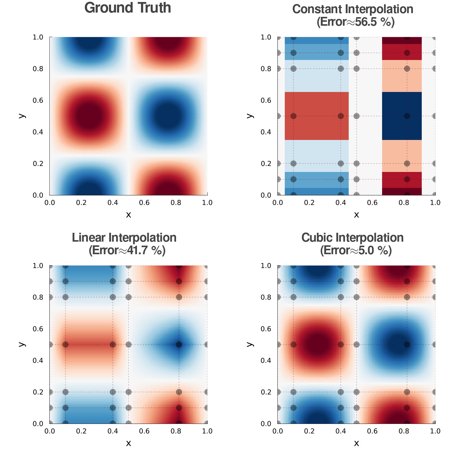
Comparison on a non-uniform 2D rectilinear grid for $f(x, y) = \sin(2\pi x) \cos(2\pi y)$. Cubic interpolation maintains high accuracy and captures extrema even on coarse, non-uniform grids. The gray dots in the image below represent the given node points (6x7 grid), and the dashed lines illustrate the grid structure.

Performance

Benchmark comparison against Interpolations.jl, DataInterpolations.jl, and Dierckx.jl for cubic spline interpolation.

Env: Local · macOS 15.7.3 · Apple M1 Pro · Julia 1.13.1
Pkg: FastInterpolations (v0.4.20) · Interpolations (v0.16.3) · DataInterpolations (v10.1.3) · Dierckx (v0.5.4)

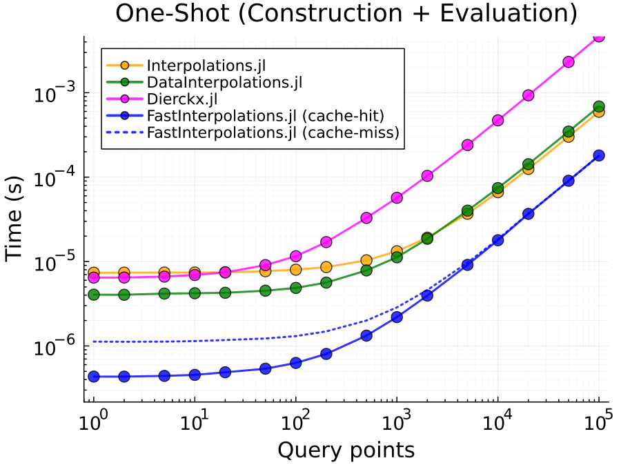
Speedup: (3.3 ~ 17.0)× vs Interpolations.jl · (3.8 ~ 9.4)× vs DataInterpolations.jl · (14.9 ~ 26.3)× vs Dierckx.jl

One-shot (construction + evaluation) time per call with fixed grid size $n=100$. FastInterpolations.jl is significantly faster even on the first call (cache-miss), and becomes even faster on subsequent calls (cache-hit).

More Features

Analytic Derivatives

Exact 1st–3rd order derivatives from spline coefficients — no finite differences. ND interpolants support gradient, hessian, and laplacian, plus jacobian for vector-valued data.

# 1D example
cubic_interp(x, y, 5.0; deriv=DerivOp(1))   # 1D: f'(x)

# 2D example 
itp2d = cubic_interp((x, y), data2D)

point = (0.5, 1.0)                       # query point (x, y)
itp2d(point; deriv=DerivOp(1, 0))        # ∂f/∂x
itp2d(point; deriv=DerivOp(1, 1))        # ∂²f/∂x∂y (mixed partial)
gradient(itp2d, point)                   # (∂f/∂x, ∂f/∂y)
hessian(itp2d, point)                    # 2×2 Hessian matrix

📖 1D Derivatives · ND Derivatives

Analytic Integration

Exact definite integration from spline coefficients — no numerical quadrature.

itp = cubic_interp(x, y)
integrate(itp, 0.0, π)                       # 1D: ∫₀^π f(x) dx

itp2d = cubic_interp((x, y), data2D)
integrate(itp2d, (0.0, 0.0), (1.0, 1.0))    # 2D: ∫∫ f dA over [0,1]²
integrate(itp2d)                              # 2D: full-domain integral

📖 1D Integration · ND Integration

Boundary Conditions

Rich type system for physical BCs — Neumann, periodic, polynomial fit, and custom per-endpoint.

cubic_interp(x, y, xq; bc=CubicFit())                        # cubic polynomial fit (default)
cubic_interp(x, y, xq; bc=PeriodicBC())                      # C²-continuous periodic
cubic_interp(x, y, xq; bc=BCPair(Deriv1(2.0), Deriv1(0.0)))  # Neumann: specify f' at each end
cubic_interp(x, y, xq; bc=BCPair(Deriv1(2.0), Deriv2(0.0)))  # mixed: slope left, curvature right

📖 Boundary Conditions Guide

Extrapolation

Queries outside the data domain throw DomainError by default. Use Extrap() to allow them:

cubic_interp(x, y; extrap=Extrap(:clamp))             # clamp to boundary value
cubic_interp(x, y; extrap=Extrap(:extend))            # extend boundary polynomial
cubic_interp(x, y; extrap=Extrap(:fill; fill_value=NaN)) # fill with constant value
# also :wrap (periodic) and :none (default, throws DomainError)

📖 Extrapolation Guide ·

Search

Non-uniform (Vector) grids require an interval search. The default AutoSearch() picks the best strategy per-call:

itp = linear_interp(x_vec, y_vec; search=AutoSearch())  # default, adapts per-call
itp(0.5)          # scalar → binary search
itp(sorted_xq)    # sorted detected → linear walk + binary fallback
itp(rand_xq)      # random detected → binary search
itp(0.5; search=BinarySearch())  # manual override (rarely needed)

📖 Search Policies

Hints

Give the search a positional hint to speed up lookup — enables O(1) sequential access (ODE solvers, streaming):

itp = cubic_interp(x, y)
hint = Ref(1)  # grid interval index, updated automatically
for t in time_steps  # monotonic or streaming
    val = itp(t; hint=hint)  # hint is reused & updated each call
end

📖 Using Hints

See also: Factory Functions · Complex Numbers · AutoDiff · Thread Safety · Optim.jl Integration

Documentation

For detailed guides on boundary conditions, extrapolation, and performance tuning, visit the Documentation.

License

Apache License 2.0

Contact

Min-Gu Yoo (General Atomics) [email protected]