
OishiLab/OpenMAP-T1
OishiLab/OpenMAP-T1 has 50 GitHub stars and 8 forks. GitHot measured 0 stars in 24 hours. Last checked 2026-11-15 17:25 UTC. Last push 2026-11-13.
Measured star growth
- in 24h
- 0
- in 7 days
- Update delayed
- in 15 days
- Update delayed
- in 1 month
- Update delayed
Net star changes over overlapping periods, not daily totals. Missing measurements are left blank. Stars measure attention, not software quality.
About
Whole Brain Segmentation and Parecllation Using OpenMAP-T1 Method for 3D T1 Brain MRI
Machine LearningREADME.md
Original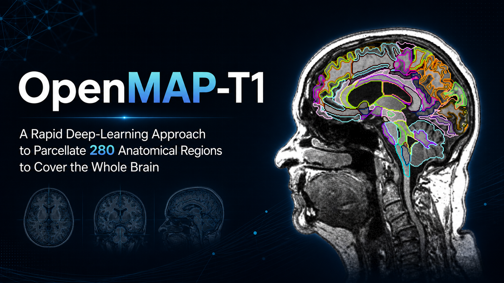
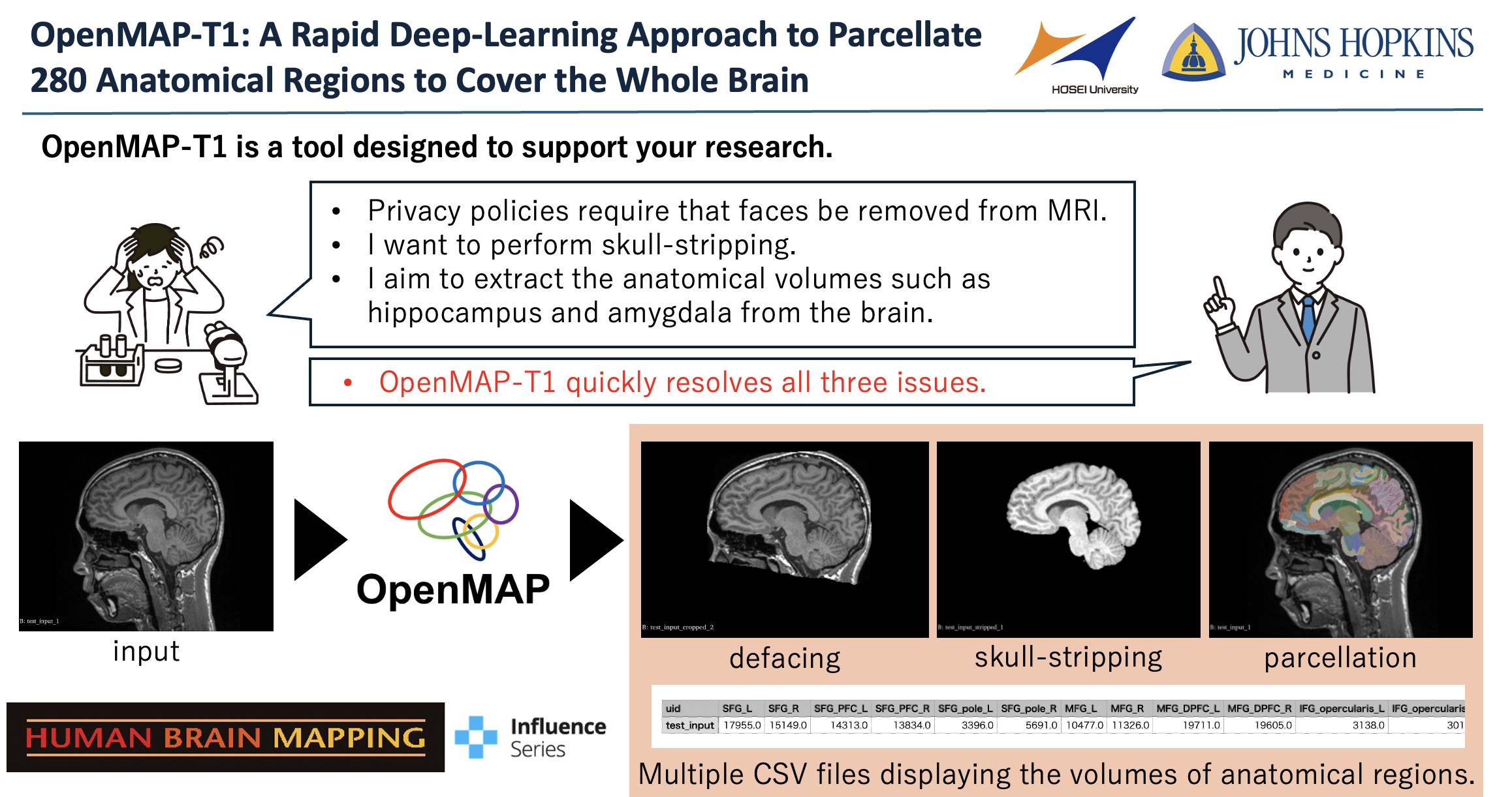
OpenMAP-T1 and OpenMAP-T1c

Languages: English | 日本語 (Japanese) | 中文 (Chinese)





OpenMAP-T1: A Rapid Deep-Learning Approach to Parcellate 280 Anatomical Regions to Cover the Whole Brain
Author: Kei Nishimaki, Kengo Onda, Kumpei Ikuta, Jill Chotiyanonta, Yuto Uchida, Susumu Mori, Hitoshi Iyatomi, Kenichi Oishi
The Russell H. Morgan Department of Radiology and Radiological Science, The Johns Hopkins University School of Medicine, Baltimore, MD, USA
Department of Applied Informatics, Graduate School of Science and Engineering, Hosei University, Tokyo, Japan
The Richman Family Precision Medicine Center of Excellence in Alzheimer's Disease, Johns Hopkins University School of Medicine, Baltimore, MD, USA
Abstract: This study introduces OpenMAP-T1, a deep learning-based method for rapid and accurate whole brain parcellation in T1-weighted brain MRI, aiming to overcome the limitations of conventional normalization-to-atlas-based approaches and multi-atlas label-fusion (MALF) techniques. Brain image parcellation is a fundamental process in neuroscientific and clinical research, enabling detailed analysis of specific cerebral regions. Normalization-to-atlas-based methods have been employed for this task, but they face limitations due to variations in brain morphology, especially in pathological conditions. The MALF techniques improved the accuracy of the image parcellation and robustness to variations in brain morphology but at the cost of high computational demand that requires lengthy processing time. OpenMAP-T1 integrates several convolutional neural network models across six phases: preprocessing, cropping, skull stripping, parcellation, hemisphere segmentation, and final merging. This process involves standardizing MRI images, isolating the brain tissue, and parcellating it into 280 anatomical structures that cover the whole brain, including detailed gray and white matter structures, while simplifying the parcellation processes and incorporating robust training to handle various scan types and conditions. The OpenMAP-T1 was tested on eight available open resources, including real-world clinical images, demonstrating robustness across different datasets with variations in scanner types, magnetic field strengths, and image processing techniques like defacing. Compared to existing methods, OpenMAP-T1 significantly reduced the processing time per image from several hours to less than 90 seconds without compromising accuracy. It was particularly effective in handling images with intensity inhomogeneity and varying head positions, conditions commonly seen in clinical settings. The adaptability of OpenMAP-T1 to a wide range of MRI datasets and robustness to various scan conditions highlight its potential as a versatile tool in neuroimaging.
Paper: https://onlinelibrary.wiley.com/doi/full/10.1002/hbm.70063
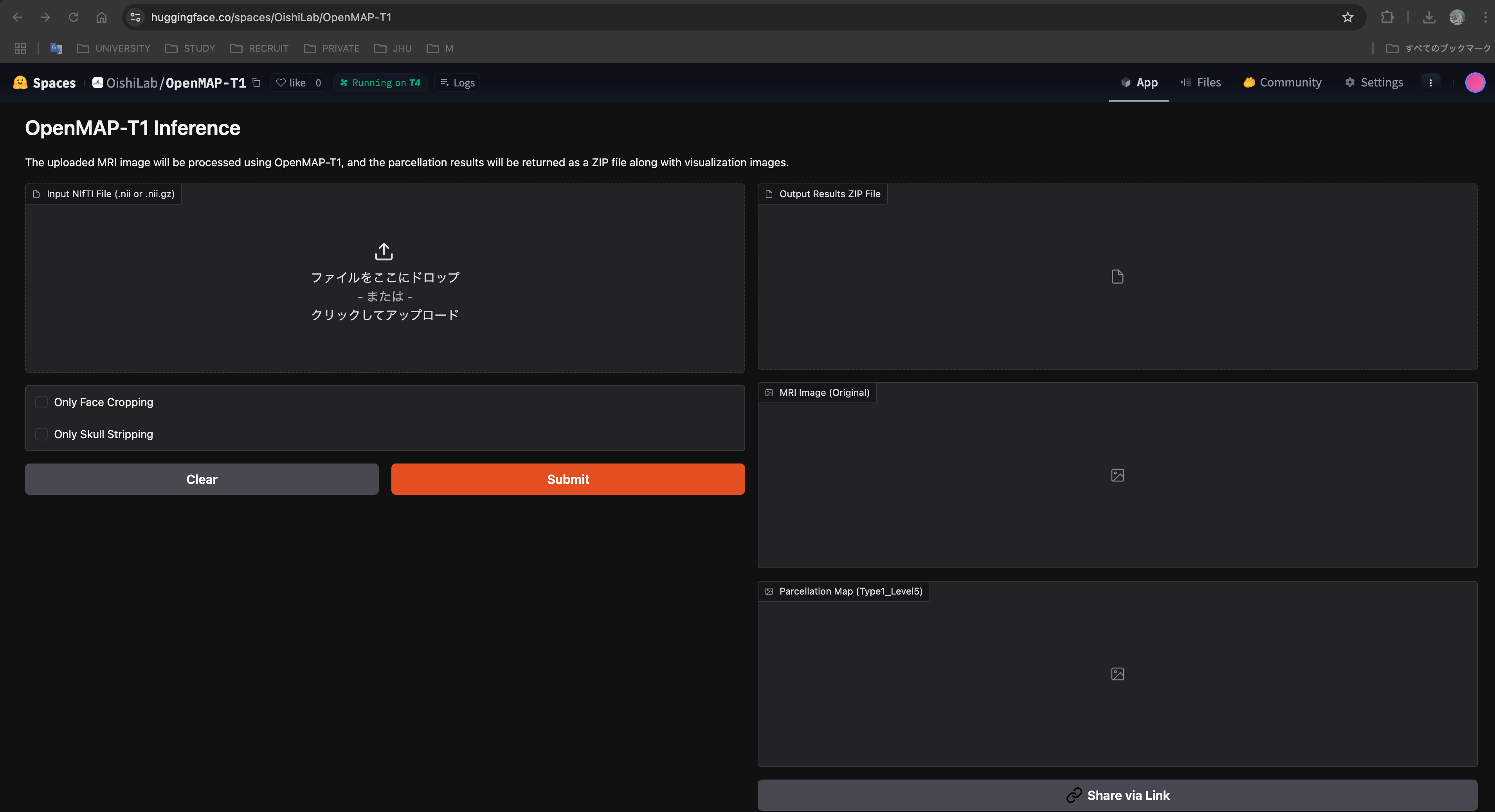
Cloud Application: https://huggingface.co/spaces/OishiLab/OpenMAP-T1
Published in Human Brain Mapping
🧠 OpenMAP series
OpenMAP is a family of deep-learning models that parcellate the whole brain into 280 anatomical regions.
- OpenMAP-T1 and OpenMAP-T1c are both included in this repository and take a T1-weighted MRI. OpenMAP-T1 is aimed at detailed parcellation of the brain parenchyma, especially white matter. OpenMAP-T1c is trained on labels registered from T2-weighted MRI and pays more attention to CSF around the cortical sulci, Sylvian fissures, and subarachnoid cisterns.
- For finer CSF segmentation from a T2-weighted MRI, use OpenMAP-T2.
📋 Requirements
- Python 3.12 or later (required by scipy 1.18). The Docker image uses Python 3.14.8, the newest release that still has PyTorch wheels.
- PyTorch 2.14 or later (installed automatically with
uv sync; install separately when using pip) - Other pinned libraries: nibabel 5.4.2, pandas 3.0.6, scipy 1.18.1, SimpleITK 2.5.6, tqdm 4.70.1
📦 Installation
OpenMAP-T1 parcellates the whole brain into 280 anatomical regions based on JHU-atlas in 50 (sec/case).
Installation with uv (Recommended)
uv is an extremely fast Python package installer and resolver written in Rust. It provides a faster alternative to pip for managing dependencies.
Install uv
Install uv using one of the following methods:macOS and Linux:
curl -LsSf https://astral.sh/uv/install.sh | shWindows:
powershell -ExecutionPolicy ByPass -c "irm https://astral.sh/uv/install.ps1 | iex"Or using pip:
pip install uvClone this repository, and go into the repository:
git clone https://github.com/OishiLab/OpenMAP-T1.git
cd OpenMAP-T1
- Install dependencies with uv (including PyTorch):
uv sync
Please apply and download the OpenMAP-T1 v3 pre-trained model from the link below and place it in
MODEL_FOLDERon your server.You can run OpenMAP-T1!
Installation with pip (Alternative)
Install Python 3.12 or later and create a virtual environment.
Clone this repository, and go into the repository:
git clone https://github.com/OishiLab/OpenMAP-T1.git
cd OpenMAP-T1
- Install PyTorch compatible with your environment.
https://pytorch.org/
The latest stable PyTorch (2.15+) requires Python 3.11 or later; this project requires Python 3.12 or later because of scipy 1.18.
Once you select your environment, the required commands will be displayed.
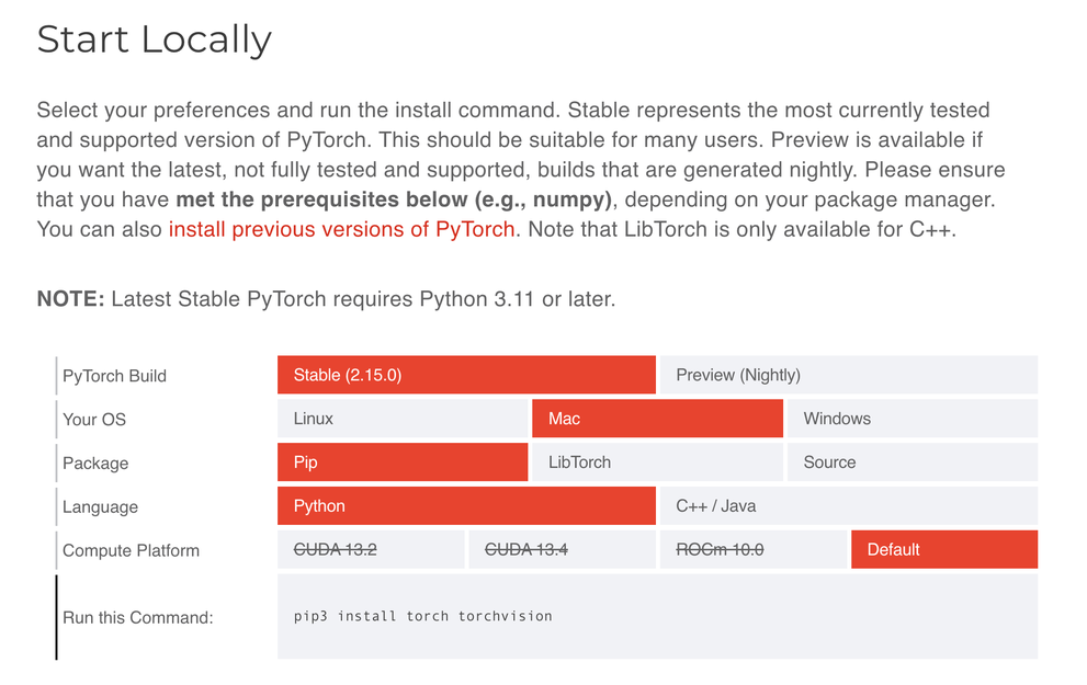
If you want to install an older PyTorch environment, you can download it from the link below.
https://pytorch.org/get-started/previous-versions/
- Install libraries other than PyTorch:
pip install -r requirements.txt
Please apply and download the OpenMAP-T1 v3 pre-trained model from the link below and place it in
MODEL_FOLDERon your server.You can run OpenMAP-T1!
🐳 Docker Installation Instruction
The Docker image is based on python:3.14.8-slim and installs dependencies from requirements_for_docker.txt, which is exported from uv.lock. To regenerate it after dependency updates, run:
uv export --no-hashes --no-emit-project --no-dev -o requirements_for_docker.txt
- Build the Docker Image
In summary, this command creates a Docker image named "openmap-t1" based on the Dockerfile and files in your current directory.
docker build -t openmap-t1 .
docker build: This command builds a Docker image using the instructions provided in the Dockerfile.-t openmap-t1: The-tflag tags the image with the name "openmap-t1". This makes it easier to refer to later..: The dot represents the build context, which means Docker will look for the Dockerfile and other necessary files in the current directory.
- Run the Docker Container
docker run --rm -it -v "$(pwd):/app" openmap-t1 -i INPUT_FOLDER -o OUTPUT_FOLDER -m MODEL_FOLDER
docker run: This starts a new container from a Docker image.--rm: Automatically removes the container when it stops running, keeping your system clean by not leaving behind stopped containers.-itCombines two options:-ikeeps STDIN open (interactive mode).-tallocates a pseudo-TTY (allows terminal-like interaction).
Together, these options let you interact with the container through your terminal if needed.
-v "$(pwd):/app": Mounts your current working directory (the result of$(pwd)) into the/appdirectory inside the container. This means:- Any files in your current folder are available inside the container under
/app. - Any changes made inside the container (like output files) will be reflected on your host system.
- Any files in your current folder are available inside the container under
openmap-t1: This is the name of the Docker image from which the container is created. It should have been built previously using a command likedocker build -t openmap-t1 ..-i INPUT_FOLDER -o OUTPUT_FOLDER -m MODEL_FOLDERThese are the command-line arguments passed to the application running inside the container:-i INPUT_FOLDER: Specifies the input folder path.-o OUTPUT_FOLDER: Specifies the output folder path.-m MODEL_FOLDER: Specifies the model folder path.
Replace
INPUT_FOLDER,OUTPUT_FOLDER, andMODEL_FOLDERwith the appropriate directory names or paths that exist within the mounted/appdirectory (for example,input,output, andmodel).
⬇️ How to download the pretrained model.
You can get the pretrained model from this link. Link of pretrained model

💻 All Commands
Using OpenMAP-T1 is straightforward. You can use it in a terminal on Linux, macOS, or Windows. We provide CPU as well as GPU support. Running on GPU is a lot faster though and should always be preferred. Here is a minimal example of how you can use OpenMAP-T1.
Basic Usage
Run the script from your terminal using:
# uv (if you installed with uv sync)
uv run python src/parcellation.py -i INPUT_FOLDER -o OUTPUT_FOLDER -m MODEL_FOLDER
# pip (activate virtual environment first: source .venv/bin/activate)
python3 src/parcellation.py -i INPUT_FOLDER -o OUTPUT_FOLDER -m MODEL_FOLDER
# Docker
docker run --rm -it -v "$(pwd):/app" openmap-t1 -i INPUT_FOLDER -o OUTPUT_FOLDER -m MODEL_FOLDER
# Save outputs as .nii (optional; default is .nii.gz)
python3 src/parcellation.py -i INPUT_FOLDER -o OUTPUT_FOLDER -m MODEL_FOLDER --output-ext .nii
- -i INPUT_FOLDER: Specifies the folder containing the input brain MRI images (or a single
.nii/.nii.gzfile). - -o OUTPUT_FOLDER: Defines the folder where the results will be saved. This folder will be created automatically if it does not exist.
- -m MODEL_FOLDER: Indicates the folder containing the pretrained models for processing (e.g.,
model/V3for OpenMAP-T1 ormodel/OpenMAP-T1cfor OpenMAP-T1c). - --mode {auto, t1, t1c}: Pipeline variant to run. Default is
auto, which automatically detectst1(142-classPNet) ort1c(139-classPNetwith sulcal CSF internal/external subdivision) from the weights in-m. - --output-ext {.nii.gz, .nii}: Output extension for generated NIfTI files. Default is
.nii.gz. - --output-space {native, conform, both}: Voxel grid for saved NIfTI outputs in
cropped/,stripped/, andparcellated/. Default isnative.native: Resample to the N4-corrected canonical input grid (default; same filenames as in earlier releases).conform: Keep the 1 mm isotropic 256³ processing grid; filenames include the_1mmsuffix.both: Write both versions; 1 mm files are saved underconform/with the_1mmsuffix.
- --batch-size: Number of 2.5D slices processed per forward pass. Default is
16. - --no-amp: Disable CUDA automatic mixed precision (run CUDA inference in full precision).
Output Space
Inference runs on a 1 mm isotropic grid internally. By default, saved parcellation maps and intermediate masks are resampled back to the N4-corrected canonical input geometry (native). To keep outputs on the 1 mm grid, or to save both grids, use --output-space:
# uv
uv run python src/parcellation.py -i INPUT_FOLDER -o OUTPUT_FOLDER -m MODEL_FOLDER --output-space conform
uv run python src/parcellation.py -i INPUT_FOLDER -o OUTPUT_FOLDER -m MODEL_FOLDER --output-space both
# pip
python3 src/parcellation.py -i INPUT_FOLDER -o OUTPUT_FOLDER -m MODEL_FOLDER --output-space conform
python3 src/parcellation.py -i INPUT_FOLDER -o OUTPUT_FOLDER -m MODEL_FOLDER --output-space both
1 mm outputs use the _1mm suffix (for example, A_Type1_Level5_1mm.nii.gz, A_cropped_mask_1mm.nii.gz). The original/ folder is always saved in the input-derived geometry. CSV regional volumes are always computed on the 1 mm grid, regardless of this option.
Optional Fast Processing Steps
OpenMAP-T1 now allows you to perform only specific processing steps using the following mutually exclusive flags. By specifying these options, OpenMAP-T1 skips unnecessary processing steps, which can significantly reduce overall processing time.
- Only Face Cropping: If you only want to perform face cropping and skip the rest of the processing steps, use:
# uv
uv run python src/parcellation.py -i INPUT_FOLDER -o OUTPUT_FOLDER -m MODEL_FOLDER --only-face-cropping
# pip
python3 src/parcellation.py -i INPUT_FOLDER -o OUTPUT_FOLDER -m MODEL_FOLDER --only-face-cropping
# Docker
docker run --rm -it -v "$(pwd):/app" openmap-t1 -i INPUT_FOLDER -o OUTPUT_FOLDER -m MODEL_FOLDER --only-face-cropping
- Only Skull Stripping: If you want to perform only skull stripping and skip all other processing steps, use the skull stripping flag. Note that skull stripping requires face cropping as a prerequisite, so face cropping is not considered one of the "other processing" steps that are skipped, use:
# uv
uv run python src/parcellation.py -i INPUT_FOLDER -o OUTPUT_FOLDER -m MODEL_FOLDER --only-skull-stripping
# pip
python3 src/parcellation.py -i INPUT_FOLDER -o OUTPUT_FOLDER -m MODEL_FOLDER --only-skull-stripping
# Docker
docker run --rm -it -v "$(pwd):/app" openmap-t1 -i INPUT_FOLDER -o OUTPUT_FOLDER -m MODEL_FOLDER --only-skull-stripping
⚡ Using GPU
OpenMAP-T1 selects CUDA automatically when a GPU is available (Using device: cuda at startup). GPU execution is much faster than CPU and is recommended whenever possible. Each run uses a single GPU.
On Linux or Windows (WSL2) with an NVIDIA GPU, install the NVIDIA Container Toolkit before using GPU inside Docker. Without --gpus, the container typically falls back to CPU even on a GPU host.
Docker example with GPU:
docker run --rm -it --gpus all -v "$(pwd):/app" openmap-t1 -i INPUT_FOLDER -o OUTPUT_FOLDER -m MODEL_FOLDER
To pin a specific GPU locally (for example, GPU 1), prepend CUDA_VISIBLE_DEVICES=N:
# uv
CUDA_VISIBLE_DEVICES=1 uv run python src/parcellation.py -i INPUT_FOLDER -o OUTPUT_FOLDER -m MODEL_FOLDER
# pip
CUDA_VISIBLE_DEVICES=1 python3 src/parcellation.py -i INPUT_FOLDER -o OUTPUT_FOLDER -m MODEL_FOLDER
The same idea in Docker (for example, host GPU 1):
docker run --rm -it --gpus '"device=1"' -v "$(pwd):/app" openmap-t1 -i INPUT_FOLDER -o OUTPUT_FOLDER -m MODEL_FOLDER
On macOS, Docker runs in a Linux VM and cannot use the host Apple Silicon GPU (MPS). Use a native install (uv or pip) on Mac for MPS acceleration, or run Docker on CPU.
If an error occurs for Windows users, please change python3 to python.
Folder
All input images must be NIfTI files (.nii or .nii.gz). By default, generated NIfTI outputs are saved as .nii.gz (use --output-ext .nii to save as .nii).
The tree below shows the default layout with --output-space native (outputs resampled to the N4-corrected canonical input grid). With --output-space conform, the same subfolder names are used, but files remain on the 1 mm grid and include _1mm in the filename (for example, A_Type1_Level5_1mm.nii.gz). With --output-space both, the native layout is written as shown, and 1 mm copies are added under conform/ (for example, conform/parcellated/A_Type1_Level5_1mm.nii.gz).
INPUT_FOLDER/
   ├ A.nii or .nii.gz
   ├ B.nii or .nii.gz
   ├ *.nii or .nii.gz

OUTPUT_FOLDER/
   ├── processing_log.txt
   ├── failed_cases.csv             # only when a case fails, is skipped, or is low_volume
   ├── A
   │   ├── cropped
   │   │   ├── A_cropped_mask.nii.gz
   │   │   └── A_cropped.nii.gz
   │   ├── csv
   │   │   ├── A_Type1_Level1.csv
   │   │   ├── A_Type1_Level2.csv
   │   │   ├── A_Type1_Level3.csv
   │   │   ├── A_Type1_Level4.csv
   │   │   ├── A_Type1_Level5.csv
   │   │   ├── A_Type2_Level1.csv
   │   │   ├── A_Type2_Level2.csv
   │   │   ├── A_Type2_Level3.csv
   │   │   ├── A_Type2_Level4.csv
   │   │   ├── A_Type2_Level5.csv
   │   │   └── A_SylvianRatio.csv   # only in OpenMAP-T1c mode (t1c)
   │   ├── original
   │   │   ├── A_N4.nii.gz
   │   │   └── A.nii.gz
   │   ├── parcellated
   │   │   ├── A_Type1_Level1.nii.gz
   │   │   ├── A_Type1_Level2.nii.gz
   │   │   ├── A_Type1_Level3.nii.gz
   │   │   ├── A_Type1_Level4.nii.gz
   │   │   ├── A_Type1_Level5.nii.gz
   │   │   ├── A_Type2_Level1.nii.gz
   │   │   ├── A_Type2_Level2.nii.gz
   │   │   ├── A_Type2_Level3.nii.gz
   │   │   ├── A_Type2_Level4.nii.gz
   │   │   └── A_Type2_Level5.nii.gz
   │   ├── stripped
   │   │   ├── A_stripped_mask.nii.gz
   │   │   └── A_stripped.nii.gz
   │   └── conform/                 # only with --output-space both
   │       ├── cropped/
   │       │   ├── A_cropped_mask_1mm.nii.gz
   │       │   └── A_cropped_1mm.nii.gz
   │       ├── parcellated/
   │       │   └── A_Type1_Level5_1mm.nii.gz
   │       └── stripped/
   │           ├── A_stripped_mask_1mm.nii.gz
   │           └── A_stripped_1mm.nii.gz
   ├── ...

MODEL_FOLDER/
   ├ CNet/CNet.pth
   ├ SSNet/SSNet.pth
   ├ PNet/PNet.pth
   └ HNet/HNet.pth
The pretrained models use one weight file per network (model/V3 for OpenMAP-T1, model/OpenMAP-T1c for OpenMAP-T1c). PNet (and HNet in OpenMAP-T1c) uses a single model for all anatomical views; orientation is encoded at inference time.
All runtime console messages (stdout, stderr, and progress logs) are automatically saved to processing_log.txt at the root of OUTPUT_FOLDER.
If any case fails, is skipped by a short-circuit flag, or yields a clearly abnormal total brain volume (default: < 10,000 mm³ on the 1 mm isotropic grid), it is listed in failed_cases.csv at the root of OUTPUT_FOLDER. Columns: case_id, input_path, status (failed, skipped, or low_volume), reason, and total_brain_volume_mm3.
🗺️ Level Metadata (JHU-Atlas)
The level/ folder contains lookup tables and hierarchy definitions related to the JHU-atlas-based parcellation, organized into level/OpenMAP-T1/ (standard OpenMAP-T1) and level/OpenMAP-T1c/ (OpenMAP-T1c with internal/external sulcal CSF and subarachnoid cistern definitions).
level/OpenMAP-T1/OpenMAP-T1_multilevel_lookup_table_dictionary.csvandlevel/OpenMAP-T1c/OpenMAP-T1c_multilevel_lookup_table_dictionary.csvinclude the official ROI names for Type1 Level5 and their corresponding multilevel mappings.- Type1 text dictionaries are named
Type1Level1.txttoType1Level5.txtinside each subfolder (level/OpenMAP-T1/andlevel/OpenMAP-T1c/).
📎 Supplementary information
 The OpenMAP-T1 parcellates the entire brain into five hierarchical structural levels, with the coarsest level comprising eight structures and the finest level comprising 280 structures.
For additional visualization and detailed analysis, you can also utilize 3D Slicer. 3D Slicer is a free, open-source platform for medical image computing that provides robust tools for segmentation, registration, and 3D visualization, making it an excellent choice for exploring the parcellation maps generated by OpenMAP-T1.
For additional visualization and detailed analysis, ROIEditor is also an excellent tool. ROIEditor is a free, open-source application specifically designed for creating and editing regions of interest (ROIs) in medical imaging. Its user-friendly interface facilitates precise segmentation and fine-tuning, making it ideal for isolating and analyzing specific regions on parcellation maps generated by OpenMAP-T1.
❓ FAQ
What are the contributions of OpenMAP-T1?
For GPUs, OpenMAP-T1 processes T1-weighted images in just 1–2 minutes. Even on CPUs, processing completes in roughly 30 minutes. Moreover, OpenMAP-T1 is highly robust against variations in imaging environments and brain atrophy.Which atlas is used in OpenMAP-T1?
OpenMAP-T1 employs the JHU atlas.Can OpenMAP-T1 be used with 2D imaging data?
Although not included in the paper, our private tests indicate that OpenMAP-T1 can also work with 2D imaging. However, using 2D data might result in some regions being lost.How much GPU memory do I need to run OpenMAP-T1?
We ran all our experiments on NVIDIA RTX3090 GPUs with 24 GB memory. For inference you will need less, but since inference is implemented by exploiting the fully convolutional nature of CNNs the amount of memory required depends on your image. A typical image should run with less than 4 GB of GPU memory consumption. If you run into out of memory problems please check the following: 1) Make sure the voxel spacing of your data is correct and 2) Ensure your MRI image only contains the head region.Can OpenMAP-T1 use Apple Silicon (MPS) on MacBook?
Yes. OpenMAP-T1 supports MPS (Metal Performance Shaders) on Apple Silicon Macs (M-series chips). When running on a MacBook with Apple Silicon, it automatically uses MPS for GPU acceleration if available, which is faster than CPU-only execution.What is the difference between OpenMAP-T1 and OpenMAP-T1c?
OpenMAP-T1 is designed for detailed parcellation of the brain parenchyma, with a particular focus on white matter structures. In contrast, OpenMAP-T1c is trained using labels registered from T2-weighted MRI, placing greater emphasis on the segmentation of perivascular and subarachnoid CSF spaces (such as cortical sulci, Sylvian fissures, and subarachnoid cisterns). If you want even more detailed and accurate CSF segmentation (when T2-weighted MRI is available), we recommend using OpenMAP-T2.
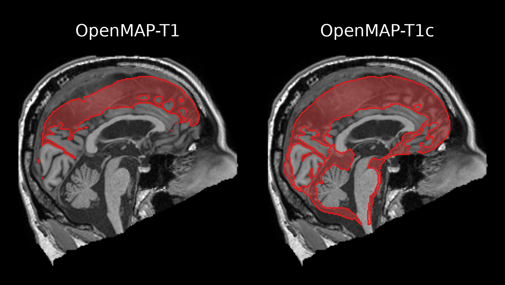
Why do some CSF labels differ between OpenMAP-T1 and OpenMAP-T1c?
The JHU atlas has continued to be extended since the MRICloud era. OpenMAP-T1 follows the conventional definition (V10B). OpenMAP-T1c uses a revised atlas in which some CSF anatomical regions have been updated, so a few CSF labels do not correspond one to one with OpenMAP-T1.What is the difference between Type 1 and Type 2?
Type 1 outputs the brain surface structure by separating it into the cortex and the subcortical white matter. Typically, Type 1 is used in most cases. In contrast, Type 2 outputs the cortex and the subcortical white matter as a single ROI. Type 2 may be employed when it is desirable to minimize the number of ROIs in data analysis or when quantifying parameters such as regional cerebral blood flow using low-resolution PET images.What units are the regional volumes in the CSV outputs, and why are they whole numbers?
Volumes are in cubic millimeters (mm³). They are reported as integers with no fractional part because they are computed as voxel counts per region on the preprocessed image that has been conformed to 1 × 1 × 1 mm isotropic spacing, so each voxel represents exactly 1 mm³. By default, saved NIfTI parcellation maps are resampled back to the N4-corrected canonical input geometry (--output-space native). Use--output-space conformorbothif you also want NIfTI files on the same 1 mm grid as the CSV volumes (filenames include_1mm).What is
{basename}_SylvianRatio.csv(e.g.,A_SylvianRatio.csv)?
Generated in OpenMAP-T1c mode (t1c), this file reports the ratio of the bilateral Sylvian fissure volume to the total sulcal CSF volume of the frontal, central, and parietal sulci:(Sylvian Fissure L+R) / (Frontal Sulcus LR + Central Sulcus LR + Parietal Sulcus LR). It is intended as a quantitative index for evaluating conditions such as Disproportionately Enlarged Subarachnoid Space Hydrocephalus (DESH) in idiopathic normal pressure hydrocephalus (iNPH).What is recorded in
failed_cases.csv?
At the end of a batch run, OpenMAP-T1 writesfailed_cases.csvunderOUTPUT_FOLDERwhen at least one case failed, was skipped by--only-face-cropping/--only-skull-stripping, or produced an abnormally small total labeled brain volume (< 10,000 mm³ by default).Will you provide the training code as well?
No. The training code is tightly wound around the data which we cannot make public.
📝 Citation
If you use OpenMAP-T1, please cite the published journal article (Human Brain Mapping, 2024), not the medRxiv preprint. Please obtain the citation from PubMed so that it matches the journal version. PubMed's Cite button provides the citation in standard styles such as APA, MLA, AMA, and NLM, so please use the one your journal or institution requires. A BibTeX entry is also provided below.
BibTeX:
@article{nishimaki2024openmap,
  author={Nishimaki, Kei and Onda, Kengo and Ikuta, Kumpei and Chotiyanonta, Jill and Uchida, Yuto and Mori, Susumu and Iyatomi, Hitoshi and Oishi, Kenichi and Alzheimer's Disease Neuroimaging Initiative and {Australian Imaging Biomarkers and Lifestyle Flagship Study of Ageing}},
  title={OpenMAP-T1: A Rapid Deep-Learning Approach to Parcellate 280 Anatomical Regions to Cover the Whole Brain},
  journal={Human Brain Mapping},
  volume={45},
  number={16},
  pages={e70063},
  keywords={brain, deep-learning, MRI, parcellation, segmentation, T1},
  doi={10.1002/hbm.70063},
  url={https://onlinelibrary.wiley.com/doi/abs/10.1002/hbm.70063},
  eprint={https://onlinelibrary.wiley.com/doi/pdf/10.1002/hbm.70063},
  note={e70063 HBM-24-0380.R2},
  abstract={ABSTRACT This study introduces OpenMAP-T1, a deep-learning-based method for rapid and accurate whole-brain parcellation in T1-weighted brain MRI, which aims to overcome the limitations of conventional normalization-to-atlas-based approaches and multi-atlas label-fusion (MALF) techniques. Brain image parcellation is a fundamental process in neuroscientific and clinical research, enabling a detailed analysis of specific cerebral regions. Normalization-to-atlas-based methods have been employed for this task, but they face limitations due to variations in brain morphology, especially in pathological conditions. The MALF techniques improved the accuracy of the image parcellation and robustness to variations in brain morphology, but at the cost of high computational demand that requires a lengthy processing time. OpenMAP-T1 integrates several convolutional neural network models across six phases: preprocessing; cropping; skull-stripping; parcellation; hemisphere segmentation; and final merging. This process involves standardizing MRI images, isolating the brain tissue, and parcellating it into 280 anatomical structures that cover the whole brain, including detailed gray and white matter structures, while simplifying the parcellation processes and incorporating robust training to handle various scan types and conditions. The OpenMAP-T1 was validated on the Johns Hopkins University atlas library and eight available open resources, including real-world clinical images, and the demonstration of robustness across different datasets with variations in scanner types, magnetic field strengths, and image processing techniques, such as defacing. Compared with existing methods, OpenMAP-T1 significantly reduced the processing time per image from several hours to less than 90 s without compromising accuracy. It was particularly effective in handling images with intensity inhomogeneity and varying head positions, conditions commonly seen in clinical settings. The adaptability of OpenMAP-T1 to a wide range of MRI datasets and its robustness to various scan conditions highlight its potential as a versatile tool in neuroimaging.},
  year={2024}
}
📚 Related Research
The following studies have utilized OpenMAP-T1 for advanced segmentation and analysis in T1-weighted MRI.
- Data-driven schizophrenia subtyping via brain atrophy trajectories and functional connectivity
Authors: Daisuke Yoshimaru, Kazuya Ouchi, Shuhei Shibukawa, Masakazu Ozawa, Motoki Hirabayashi, Ami Yuzawa, Tomokazu Tsurugizawa, Kenichi Oishi, Hirotaka James Okano;
Journal: Translational Psychiatry - Change points for dynamic biomarkers in the Alzheimer's disease pathological cascade: A 30-year cohort study
Authors: Yuto Uchida, Kei Nishimaki, Anja Soldan, Corinne Pettigrew, Sara Grace Ho, Abhay Moghekar, Mei-Cheng Wang, Michael I. Miller, Marilyn Albert, Kenichi Oishi; Journal: Alzheimer's & dementia - Acceleration of Brain Atrophy and Progression From Normal Cognition to Mild Cognitive Impairment
Authors: Yuto Uchida, MD, PhD; Kei Nishimaki; Anja Soldan, PhD; Abhay Moghekar, MBBS; Marilyn Albert, PhD; Kenichi Oishi, MD, PhD;
Journal: JAMA Network Open - A Neural Network Approach to Identify Left–Right Orientation of Anatomical Brain MRI
Authors: Kei Nishimaki; Hitoshi Iyatomi, PhD; Kenichi Oishi, MD, PhD;
Journal: Brain and Behavior - Preserved Limbic White Matter Predicts Favorable 2-Year Outcomes in Neonatal Hypoxic-Ischemic Encephalopathy
Authors: Xingyu Chen, Shuhei Tomoshige, Ria Wright, Vera J Burton, Gwendolyn Gerner, Nathanael Kuo, Jill S Chotiyanonta, Raul Chavez-Valdez, Ernest M Graham, Frances J Northington, Kenichi Oishi;
Journal: Annals of the Child Neurology Society - Utilizing routinely acquired clinical neuroimaging and electronic health record data to advance precision medicine in dementia care
Authors: Kenichi Oishi, Roy Adams, Milap A Nowrangi, Peter P Zandi, Constantine G Lyketsos;
Journal: International Review of Psychiatry