MNIST Digit Prediction - Neural Network from Scratch with NumPy

Implemented a neural network from scratch using NumPy, translating forward propagation, backpropagation, activation functions, and gradient descent into mathematical operations.

An interactive handwritten-digit classifier powered by a neural network built entirely from scratch with NumPy. No TensorFlow, no PyTorch, no high-level frameworks - just matrix math, calculus, and Python.

This README documents the complete derivation, including original handwritten notes used while developing the model.

Dataset: MNIST - 70,000 images of handwritten digits (60,000 train + 10,000 test), each 28x28 grayscale, 10 classes (0-9).

Repo: https://github.com/HelloSamved/learning-neural-network/tree/master/mnist_prediction

---

Table of Contents

• Overview
• Results
• Features
• Network Architecture
• How It Works
• Math Behind the Code
• Handwritten Derivation Notes
• Project Structure
• Getting Started
• Usage
• Training Details
• Future Improvements
• Acknowledgements
• License

---

Overview

This project builds a 3-layer fully-connected neural network (Multilayer Perceptron) to classify MNIST digits:

• Input: flattened 28x28 image = 784 values, normalized from [0,255] to [0,1]
• Hidden layers: 2 layers with 28 neurons each, sigmoid activation
• Output layer: 10 neurons (one per digit), sigmoid / softmax activation
• Training: full-batch gradient descent with backpropagation derived by hand

Everything - forward pass, loss, gradients, weight updates - is written explicitly with NumPy.

---

Results

Final training run:

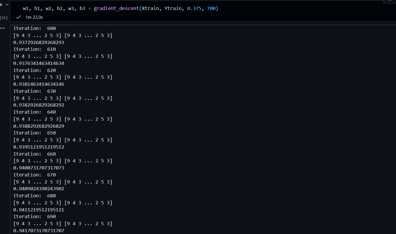
w1, b1, w2, b2, w3, b3 = gradient_descent(Xtrain, Ytrain, 0.375, 700)
Iteration 690: accuracy = 0.9417

• Training accuracy: ~94.1 percent after 700 iterations, learning rate 0.375
• Validation accuracy: ~94.7 percent (see web_interface.py / mnist_weights.npz)
• Inference: pretrained weights included, no retraining needed for demo

Training log screenshot:

---

Features

• Neural network from scratch using only NumPy, Pandas, and mathematics
• Forward propagation, backpropagation, and gradient descent implemented manually
• 784 -> 28 -> 28 -> 10 dense architecture
• Binary cross-entropy / categorical loss with chain-rule gradients
• Pretrained weights (mnist_weights.npz) for fast inference
• Streamlit web interface: upload images, confidence visualization, MNIST sample explorer
• Preprocessing: centering, normalization to 28x28 inputs
• Fully documented math + original handwritten derivations (see below)

---

Network Architecture

Input (784) -> Hidden Layer 1 (28, sigmoid) -> Hidden Layer 2 (28, sigmoid) -> Output (10, sigmoid)

Shapes (m = number of examples):

Variable	Shape	Description
X	(784, m)	Input images, flattened and normalized
W1	(28, 784)	Weights layer 1
b1	(28, 1)	Bias layer 1
A1	(28, m)	Activation layer 1
W2	(28, 28)	Weights layer 2
b2	(28, 1)	Bias layer 2
A2	(28, m)	Activation layer 2
W3	(10, 28)	Weights layer 3
b3	(10, 1)	Bias layer 3
A3	(10, m)	Output probabilities

Total trainable parameters: (28784 + 28) + (2828 + 28) + (10*28 + 10) = 23,082

---

How It Works

1. Preprocessing:

   • Load train.csv / test.csv
   • Divide pixels by 255.0 to get range [0,1]
   • Flatten each 28x28 image to vector of length 784
   • One-hot encode labels for training, keep integer labels for evaluation

2. Forward propagation: compute Z = W dot A_prev + b, then A = sigmoid(Z) layer by layer.

3. Compute loss (binary cross-entropy averaged over m examples).

4. Backpropagation: apply chain rule from output backwards to compute dW1, db1, dW2, db2, dW3, db3.

5. Gradient descent: W = W - alpha * dW, b = b - alpha * db, repeat for N iterations.

6. Prediction: predicted class = argmax(A3, axis=0).

---

Math Behind the Code

All equations use plain notation so they render correctly everywhere. Here:

• Wk = weights of layer k, bk = bias of layer k
• Zk = linear output of layer k, Ak = activation of layer k
• Y = true labels (one-hot), m = number of examples
• sigmoid(z) = 1 / (1 + exp(-z))
• f'(z) = derivative of activation

1. Forward Propagation

General rule for layer k:

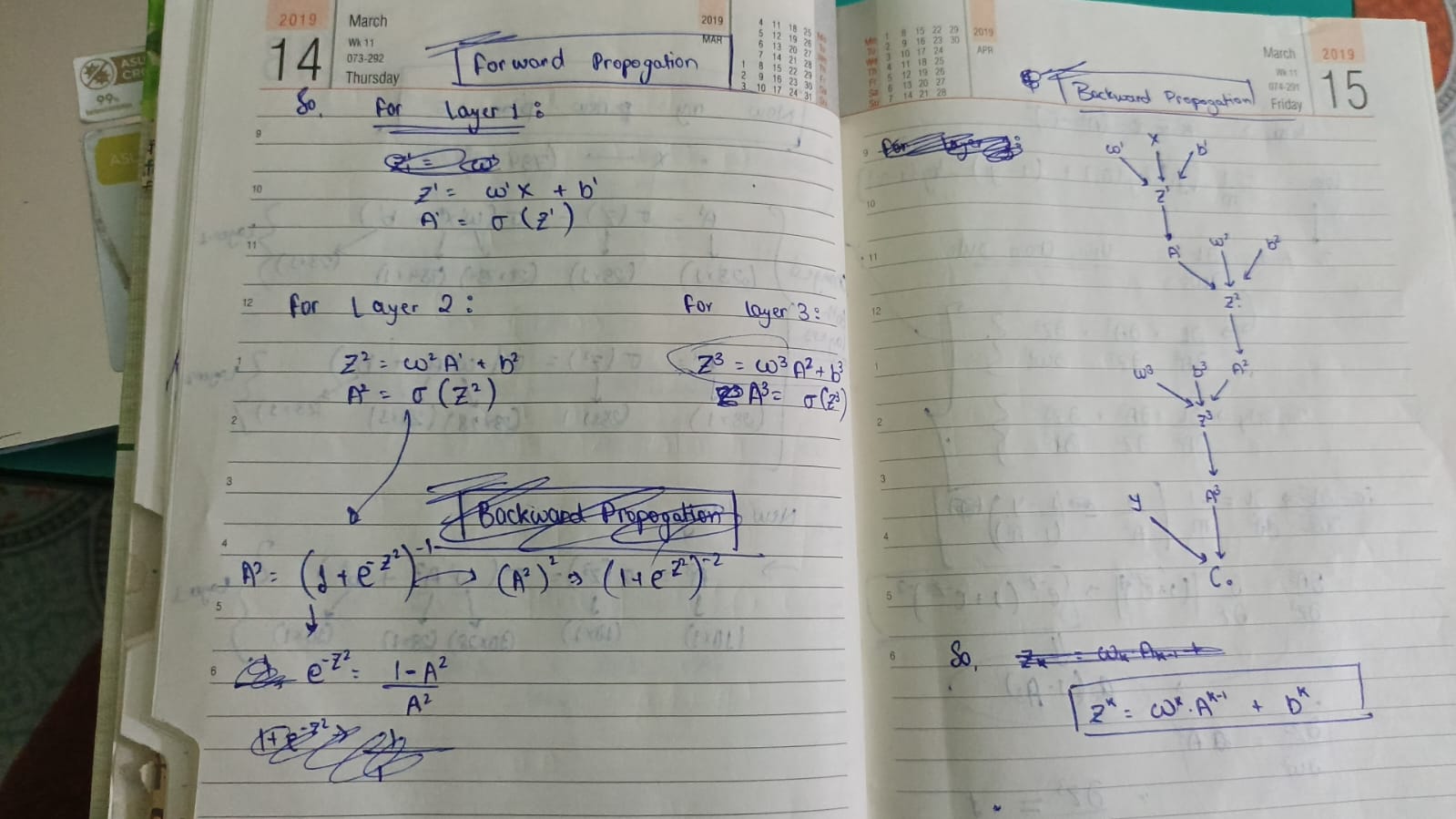
Zk = Wk dot A(k-1) + bk
Ak = sigmoid(Zk)

Expanded for this network (A0 = X):

Z1 = W1 dot X + b1
A1 = sigmoid(Z1)

Z2 = W2 dot A1 + b2
A2 = sigmoid(Z2)

Z3 = W3 dot A2 + b3
A3 = sigmoid(Z3)

Python (NumPy):

def sigmoid(z):
    return 1 / (1 + np.exp(-z))

Z1 = np.dot(W1, X) + b1
A1 = sigmoid(Z1)

Z2 = np.dot(W2, A1) + b2
A2 = sigmoid(Z2)

Z3 = np.dot(W3, A2) + b3
A3 = sigmoid(Z3)

2. Loss Function

Binary cross-entropy (averaged over m examples):

Loss = -(1/m) * sum( Y * log(A3) + (1 - Y) * log(1 - A3) )

m = X.shape[1]
loss = -(1/m) * np.sum(Y * np.log(A3 + 1e-8) + (1 - Y) * np.log(1 - A3 + 1e-8))

3. Activation Derivative

sigmoid(z) = 1 / (1 + exp(-z))
dA/dZ = A * (1 - A)

def sigmoid_derivative(A):
    return A * (1 - A)

4. Backpropagation (Chain Rule)

Output layer error term:

dZ3 = A3 - Y
dW3 = (1/m) * dot(dZ3, A2.T)
db3 = (1/m) * sum(dZ3, axis=1, keepdims=True)

Hidden layer 2:

dZ2 = dot(W3.T, dZ3) * A2 * (1 - A2)
dW2 = (1/m) * dot(dZ2, A1.T)
db2 = (1/m) * sum(dZ2, axis=1, keepdims=True)

Hidden layer 1:

dZ1 = dot(W2.T, dZ2) * A1 * (1 - A1)
dW1 = (1/m) * dot(dZ1, X.T)
db1 = (1/m) * sum(dZ1, axis=1, keepdims=True)

That is the full chain:

dL/dW1 = (dL/dA3) * (dA3/dZ3) * (dZ3/dA2) * (dA2/dZ2) * (dZ2/dA1) * (dA1/dZ1) * (dZ1/dW1)

Final compact summary (as derived in notes):

dZ3 = (A3 - Y)
dW3 = (1/m) * dZ3 dot A2.T
db3 = (1/m) * sum(dZ3)

dZ2 = W3.T dot dZ3 * f2'(Z2)
dW2 = (1/m) * dZ2 dot A1.T
db2 = (1/m) * sum(dZ2)

dZ1 = W2.T dot dZ2 * f1'(Z1)
dW1 = (1/m) * dZ1 dot X.T
db1 = (1/m) * sum(dZ1)

5. Gradient Descent Update

Wk = Wk - alpha * dWk
bk = bk - alpha * dbk

W1 -= learning_rate * dW1
b1 -= learning_rate * db1
W2 -= learning_rate * dW2
b2 -= learning_rate * db2
W3 -= learning_rate * dW3
b3 -= learning_rate * db3

Used in this project: alpha = 0.375, iterations = 700.

Weight initialization (small random values):

np.random.seed(42)
W1 = np.random.randn(28, 784) * 0.01
b1 = np.zeros((28, 1))
W2 = np.random.randn(28, 28) * 0.01
b2 = np.zeros((28, 1))
W3 = np.random.randn(10, 28) * 0.01
b3 = np.zeros((10, 1))

---

Handwritten Derivation Notes

These are the original diary notes used to derive the network. They are kept in mnist_prediction/assets/ and linked below.

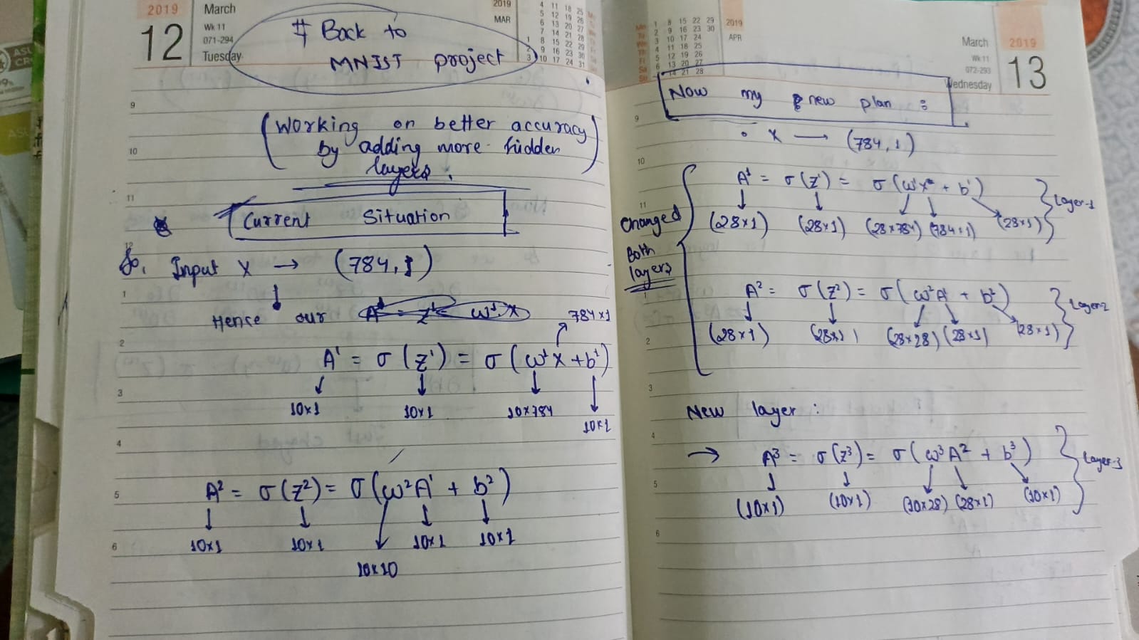
Note 1 - Architecture plan: from 2 layers to 3 layers

Working on better accuracy by adding more hidden layers. Current: Input X (784,1). New plan: X (784,1) -> A1 (28,1) -> A2 (28,1) -> A3 (10,1).

What it shows:

A1 = sigmoid(Z1) = sigmoid(W1 dot X + b1)
A2 = sigmoid(Z2) = sigmoid(W2 dot A1 + b2)
A3 = sigmoid(Z3) = sigmoid(W3 dot A2 + b3)

with shapes W1:(28,784), W2:(28,28), W3:(10,28).

Note 2 - Forward and backward propagation setup

Defines forward equations per layer and sets up the computation graph for backprop: X,b1 -> Z1 -> A1, with W2,b2 -> Z2 -> A2, with W3,b3 -> Z3 -> A3, with Y -> Cost C. General rule: Zk = Wk dot A(k-1) + bk.

Note 3 and 4 - Chain rule for output layer (W3, b3)

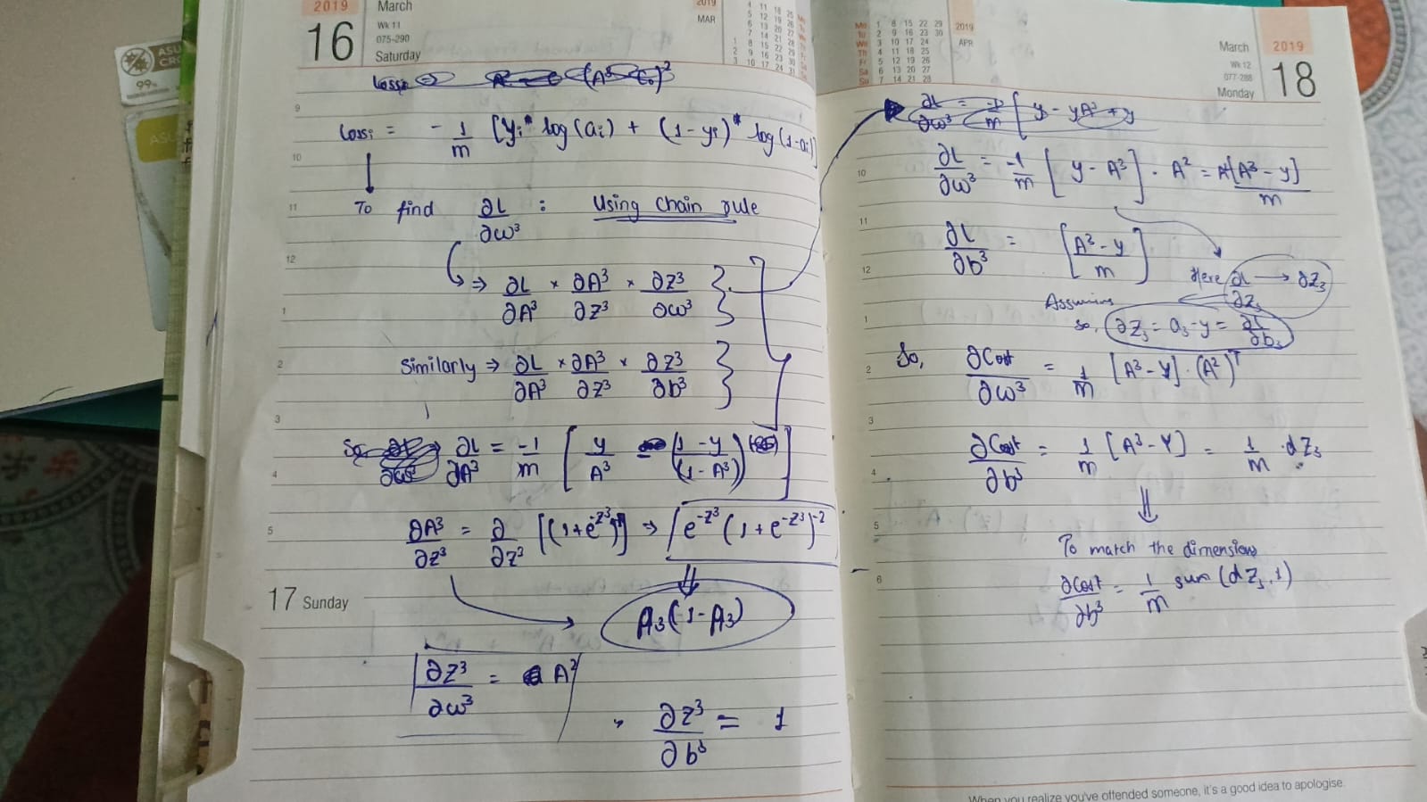
Loss:

Loss = -(1/m) * [ Y * log(A3) + (1-Y) * log(1-A3) ]

Derivation:

dL/dW3 = (dL/dA3) * (dA3/dZ3) * (dZ3/dW3)
dL/db3 = (dL/dA3) * (dA3/dZ3) * (dZ3/db3)

where:

dL/dA3 = -(1/m) * [ Y/A3 - (1-Y)/(1-A3) ]
dA3/dZ3 = A3 * (1-A3)
dZ3/dW3 = A2,  dZ3/db3 = 1

Simplified result:

dZ3 = A3 - Y
dW3 = (1/m) * dZ3 dot A2.T
db3 = (1/m) * sum(dZ3)

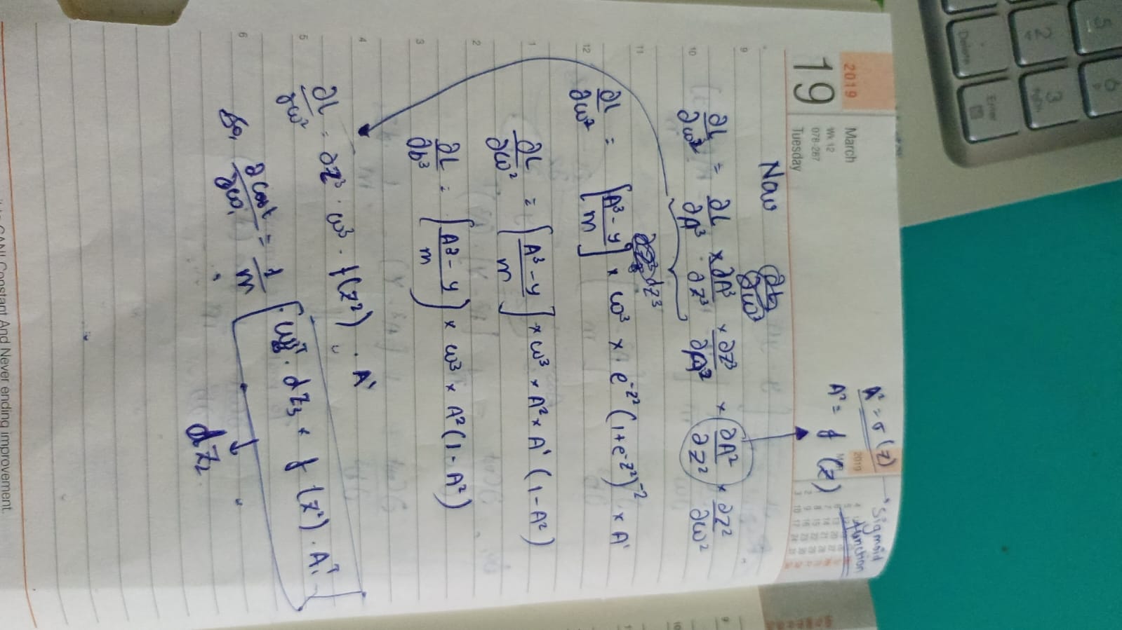
Note 5 - Hidden layer 2 gradients (W2, b2)

dL/dW2 = (dL/dA3)*(dA3/dZ3)*(dZ3/dA2)*(dA2/dZ2)*(dZ2/dW2)
dZ2 = W3.T dot dZ3 * f'(Z2)
dW2 = (1/m) * dZ2 dot A1.T
db2 = (1/m) * sum(dZ2)

Explains dimension matching of LHS and RHS by summing over axis=1.

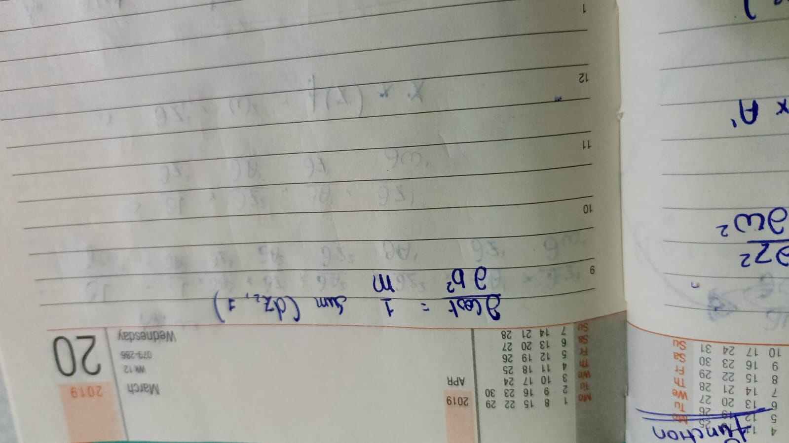
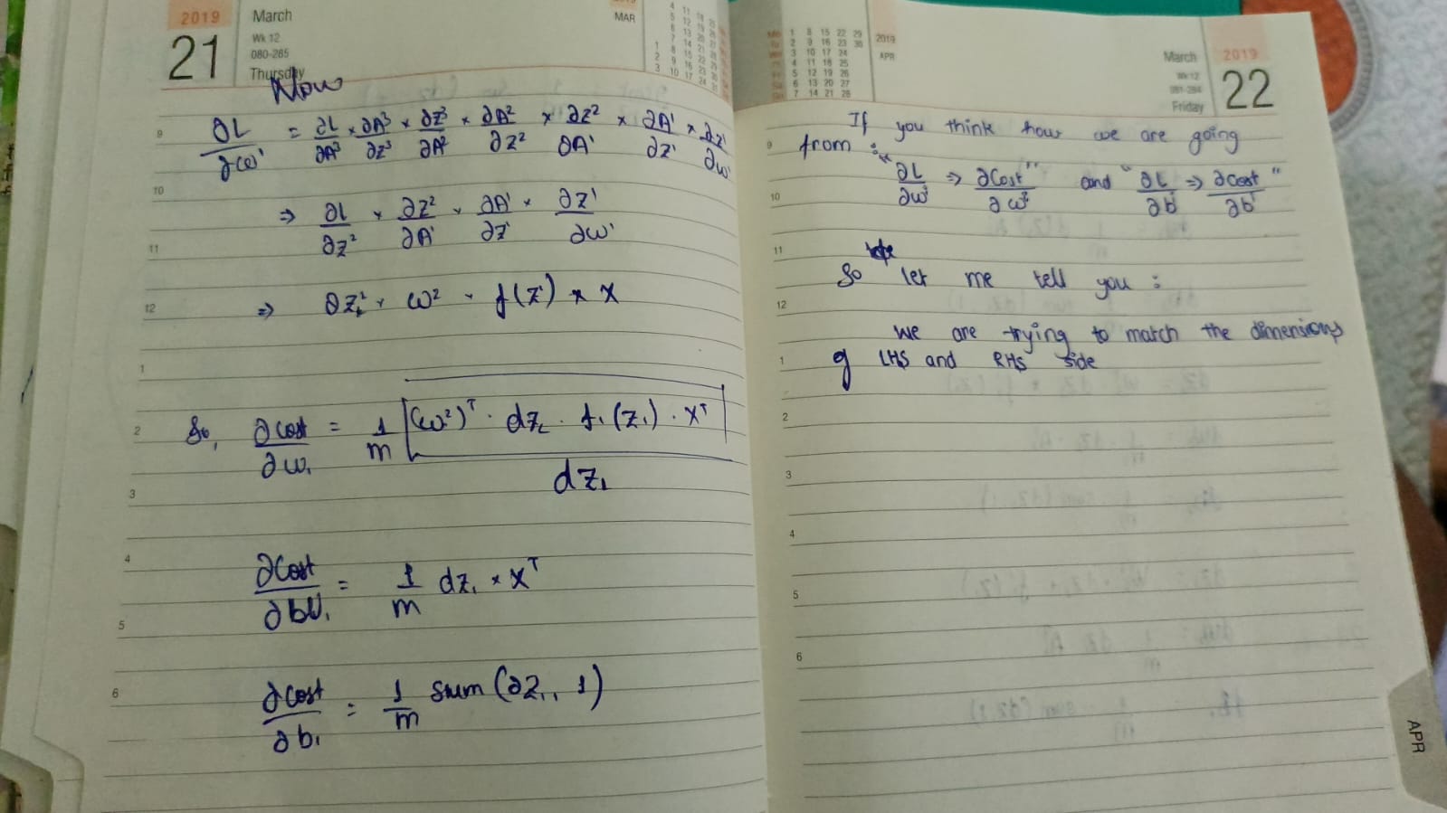
Note 6 - Hidden layer 1 gradients (W1, b1)

dL/dW1 = (dL/dZ2)*(dZ2/dA1)*(dA1/dZ1)*(dZ1/dW1)
dZ1 = W2.T dot dZ2 * f'(Z1)
dW1 = (1/m) * dZ1 dot X.T
db1 = (1/m) * sum(dZ1)

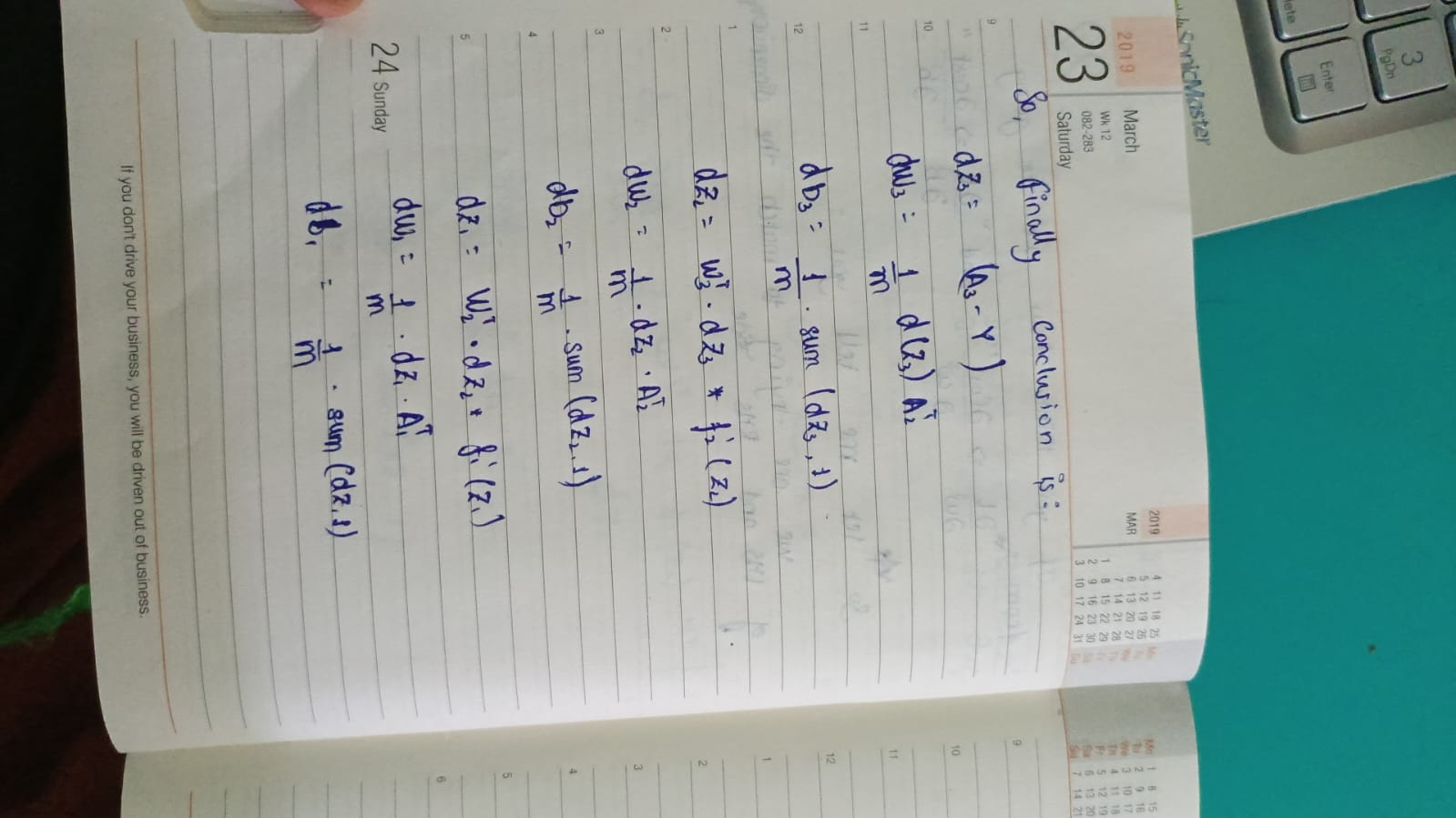
Note 7 - Final conclusion (all update equations)

Complete set used in code:

dZ3 = (A3 - Y)
dW3 = (1/m) * dZ3 dot A2.T
db3 = (1/m) * sum(dZ3, axis=1)

dZ2 = W3.T dot dZ3 * f2'(Z2)
dW2 = (1/m) * dZ2 dot A1.T
db2 = (1/m) * sum(dZ2, axis=1)

dZ1 = W2.T dot dZ2 * f1'(Z1)
dW1 = (1/m) * dZ1 dot X.T
db1 = (1/m) * sum(dZ1, axis=1)

Source folder: https://github.com/HelloSamved/learning-neural-network/tree/master/mnist_prediction/assets

---

Project Structure

mnist_prediction/
  mnist_prediction.ipynb        # original model exploration and learning notebook
  mnist-prediction.ipynb        # alternate / full training notebook
  mnist_prediction.py           # corrected reusable neural-network + preprocessing code
  mnist_prediction_pytorch.ipynb# PyTorch comparison version
  web_interface.py              # Streamlit app: upload, confidence chart, sample explorer
  mnist_weights.npz             # pretrained W1,b1,W2,b2,W3,b3 + accuracy metadata
  mnist_samples.npz             # lightweight sample set for live explorer
  train.csv                     # MNIST training data (if present locally, not committed)
  assets/
    1.jpeg                      # handwritten note: architecture
    2.jpeg                      # handwritten note: forward/backward setup
    3.jpeg                      # handwritten note: loss + chain rule
    4.jpeg                      # handwritten note: dW3, db3 derivation
    5.jpeg                      # handwritten note: dW2, db2 derivation
    6.jpeg                      # handwritten note: dW1, db1 derivation
    7.jpeg                      # handwritten note: final equations
    accuracy_image.png          # training log screenshot

---

Getting Started

Prerequisites

• Python 3.8+
• pip

1. Clone the repository

git clone https://github.com/HelloSamved/learning-neural-network.git
cd learning-neural-network/mnist_prediction

2. Install dependencies

pip install -r requirements.txt

Minimum requirements:

numpy>=1.21.0
pandas>=1.3.0
matplotlib>=3.4.0
streamlit>=1.20.0
scikit-learn>=1.0.0

3. Get MNIST data

Option A - Kaggle CSV (used in notebooks):

1. Download from https://www.kaggle.com/datasets/oddrationale/mnist-in-csv
2. Place train.csv and test.csv next to mnist_prediction.py

Option B - Auto-download with sklearn (no CSV needed):

from sklearn.datasets import fetch_openml
X, y = fetch_openml('mnist_784', version=1, return_X_y=True, as_frame=False)

---

Usage

Run the web app (recommended)

streamlit run web_interface.py

Features: upload your own digit image, see predicted digit + confidence bar chart, browse real MNIST samples.

Retrain from scratch

python mnist_prediction.py

Or in Python:

from mnist_prediction import gradient_descent, predict
import numpy as np

# Xtrain shape (784, m), Ytrain one-hot shape (10, m)
w1, b1, w2, b2, w3, b3 = gradient_descent(Xtrain, Ytrain, learning_rate=0.375, iterations=700)

pred = predict(Xtest, w1, b1, w2, b2, w3, b3)
acc = np.mean(pred == Ytest_labels)
print(f"Test accuracy: {acc * 100:.2f}%")

Predict a single image

import numpy as np
from PIL import Image
from mnist_prediction import predict_single

img = Image.open("my_digit.png").convert("L").resize((28, 28))
x = (255 - np.array(img)).reshape(784, 1) / 255.0  # invert if white background
label, probs = predict_single(x, w1, b1, w2, b2, w3, b3)
print(f"Predicted: {label}, confidence: {np.max(probs)*100:.1f}%")

Note: MNIST digits are white on black. If you draw black on white, invert the image as above.

---

Training Details

• Architecture: 784 -> 28 -> 28 -> 10
• Activation: sigmoid for all layers
• Loss: cross-entropy
• Optimizer: batch gradient descent
• Learning rate: 0.375
• Iterations: 700
• Initialization: random * 0.01, biases zero, seed 42 for reproducibility
• Preprocessing: pixels / 255.0, flatten to (784, m)

Observed progression (see accuracy_image.png):

Iteration 600: ~0.9372
Iteration 650: ~0.9395
Iteration 690: ~0.9417

Tips:

• Increase hidden units to 64 or 128 for higher accuracy, slower training
• Lower learning rate to 0.1-0.2 if loss oscillates
• Switch hidden activation to ReLU + He init + softmax output for faster convergence

---

Future Improvements

• Add ReLU + Softmax + Adam variant for comparison
• Add CNN with NumPy for 99 percent+ accuracy
• Add confusion matrix and per-digit precision/recall
• Add live drawing canvas in Streamlit app
• Export model to ONNX

---

Acknowledgements

• MNIST Database - Yann LeCun, Corinna Cortes, Christopher Burges: http://yann.lecun.com/exdb/mnist/
• Michael Nielsen - Neural Networks and Deep Learning: http://neuralnetworksanddeeplearning.com/
• 3Blue1Brown - Neural Networks series for visual intuition
• Handwritten notes in assets/ by the project author, derived March 2019

---

HELLOOOOOO If you found this helpful, please star the repo: https://github.com/HelloSamved/learning-neural-network