
hyoseokp/TorchFDTD has 28 GitHub stars and 4 forks. GitHot measured 0 stars in 24 hours and +2 in 7 days. Last checked 2026-11-21 08:31 UTC. Last push 2026-11-13.
できること
- Native CUDA engine. Fused Yee and CPML kernels, CUDA Graphs, FP32/FP64, complex Bloch fields, CPU fallback.
- Browser workbench. Objects tree, XY/XZ/YZ and perspective CAD views, materials, simulation region, layout/analysis modes, field viewer, monitor traces, Python export.
- Python first. One Project JSON shared with the browser, BatchRunner for independent cases across processes and GPUs with resume, run_tensor_batch for many structures in one CUDA launch, seeded differential evolution.
- Inverse design. Checkpointed and reversible Torch adjoints for dielectric, dispersive (ADE), Bloch, CPML, PEC/PMC, density, polygon/spline shape and source-waveform parameters. Objectives on point signals, plane spectra, N-port S-parameters, far-field and near-zone projections.
計測したスター増加
- 24時間
- 0
- 7日間
- +2
- 15日間
- 履歴を収集中
- 1か月
- 履歴を収集中
期間ごとの純増数です。期間は重複しており、日別の値ではありません。未計測の値は空欄です。スター数は注目度の指標であり、品質の保証ではありません。
概要
GPU FDTD for photonics: browser CAD workbench, Python project API and Torch-differentiable simulations on CUDA
機械学習README.md
オリジナルTorchFDTD



https://github.com/user-attachments/assets/021d317c-bd63-4019-8391-9211d9be4166
Also on YouTube: TorchFDTD Explained: GPU-Accelerated FDTD for Inverse Design.
Open-source GPU FDTD for photonics, with PyTorch gradients and a browser workbench. MIT licensed.
Build a device in Python or in the browser, simulate its electromagnetic fields, and use discrete adjoints with PyTorch autograd for inverse design. AI agents can drive it through the bundled MCP server and the agent guide.
It covers waveguides and splitters, ring resonators, photonic crystals, gratings, metasurfaces and metalenses in 2D and 3D. It runs natively on Windows and Linux, on NVIDIA GPUs through PyTorch with a CPU fallback, and is validated against analytic solutions, Mie theory, Meep, FDTDX, BeamZ and RCWA (records).
If TorchFDTD is useful to you, a GitHub star helps other researchers find it.
Quick start · Adjoint inverse design · Paper designs · Examples · Validation · Documentation · Paper
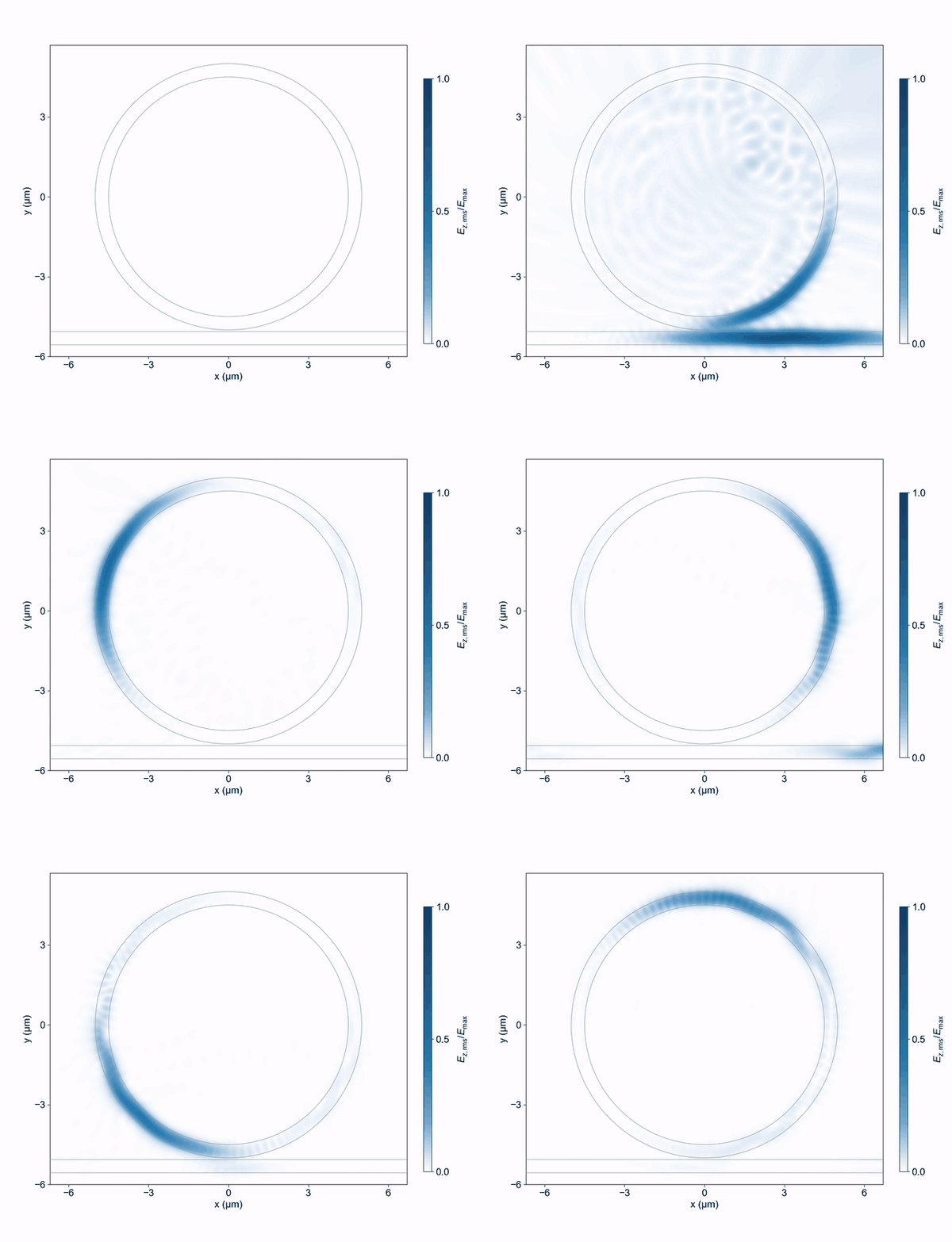
A pulse couples into a microring, circulates and leaks back into the bus waveguide. Actual 2D FDTD, showing optical-cycle RMS Ez with a fixed color scale. Full-resolution video · Model and reproduction.
- Run on your NVIDIA GPU. Fused CUDA kernels and CUDA Graphs accelerate field updates. CPU execution is available too.
- Differentiate your simulation. Discrete adjoints connect material, geometry and source parameters to PyTorch autograd.
- Work in Python or the browser. Both use the same project format. Save a browser-built device and run it from Python, or open a Python-built project in the workbench.
Quick start
Install and open the workbench
Install from PyPI with Python 3.10 or 3.12 and start the workbench:
pip install torchfdtd
torchfdtd serve
The package includes the browser workbench, so you do not need Node.js or a source checkout. Open http://127.0.0.1:8765 after starting the server.
NVIDIA GPU installation on Windows / PowerShell
Select a CUDA-enabled PyTorch build and install the cuda-kernels extra:
python -m venv torchfdtd-env
torchfdtd-env/Scripts/python.exe -m pip install torch --index-url https://download.pytorch.org/whl/cu126
torchfdtd-env/Scripts/python.exe -m pip install "torchfdtd[cuda-kernels]"
torchfdtd-env/Scripts/torchfdtd doctor
torchfdtd-env/Scripts/torchfdtd serve
torchfdtd doctor checks the installation, CUDA device and fused-kernel launch before you start.
For a CPU-only installation, use the PyTorch index https://download.pytorch.org/whl/cpu and omit [cuda-kernels] from the installation command. The cuda-kernels extra installs CuPy for the fused CUDA path. See installation and tested versions for requirements and troubleshooting.
The server listens on loopback only. Use SSH forwarding for a remote GPU. The default workbench limit is 8 million resident cells. For larger local projects, see memory admission and server limits.
Run from Python
This example runs a 3D waveguide on the fused CUDA path and saves both the project and its result:
from torchfdtd import Project, Region, Structure, Source, Monitor, Simulation

project = Project(
    name="My waveguide",
    region=Region(dimension="3d", size=(8, 6, 2), mesh=0.05, steps=1000,
                  backend="cuda", cuda_kernel="fused"),
    structures=[Structure(name="core", size=(8, 0.65, 0.4))],
    sources=[Source(center=(-2.5, 0, 0), wavelength=1.55)],
    monitors=[Monitor(name="output", center=(2, 0, 0))],
)
project.save("project.json")          # opens in the browser
result = Simulation(project).run()
result.save("results/run.npz")
Lengths are in µm and time arrays in seconds. dimension defaults to "2d" and cuda_kernel to "torch", so this example selects both explicitly. It needs an NVIDIA GPU and the cuda-kernels extra. Project.load() runs browser-made scenes.
2D example for CPU or GPU, with result loading
The 2D default runs on any install:
from torchfdtd import Project, Structure, Source, Monitor, Simulation, Result

project = Project(name="Any install", structures=[Structure(name="core", size=(8, 0.65, 0.4))],
                  sources=[Source(center=(-2.5, 0, 0), wavelength=1.55)],
                  monitors=[Monitor(name="output", center=(2, 0, 0))])
result = Simulation(project).run()    # 2D, on the CPU or the CUDA device torch reports
result.save("results/first.npz")
print(Result.load("results/first.npz").summary["backend"])
Develop from a source checkout
Clone the repository and enter its directory first. Node.js 20.19+ / 22.12+ is needed to rebuild the browser assets:
git clone https://github.com/hyoseokp/TorchFDTD.git
cd TorchFDTD
python -m venv --system-site-packages .venv
.venv/Scripts/python.exe -m pip install -e ".[dev,cuda-kernels]"
npm.cmd ci
npm.cmd run build
.venv/Scripts/python.exe -m torchfdtd.cli serve
This route reuses packages available in the base Python environment. Install a suitable PyTorch build first. The installation guide also covers wheel builds and clean-install checks.
Use from an AI agent
AGENTS.md tells coding agents when TorchFDTD fits a request, which example to start from, how to check a simulation and how to cite it. The mcp extra adds a Model Context Protocol server with tools to fetch example projects, validate and run them, normalise flux against a reference, and export Python scripts:
pip install "torchfdtd[mcp]"
torchfdtd mcp          # stdio server; register this command in any MCP client
In Claude Code, install the plugin, which adds a simulation skill and the MCP server:
/plugin install torchfdtd --marketplace hyoseokp/TorchFDTD
Adjoint inverse design
Start with a small 2D wavelength splitter: one input waveguide → square dielectric design region → two output waveguides, with 1.31 µm routed to the upper guide and 1.55 µm to the lower guide. The three guides stay fixed while TorchFDTD's discrete adjoint, computed for both wavelengths in one run, optimizes the dielectric pattern inside the square.
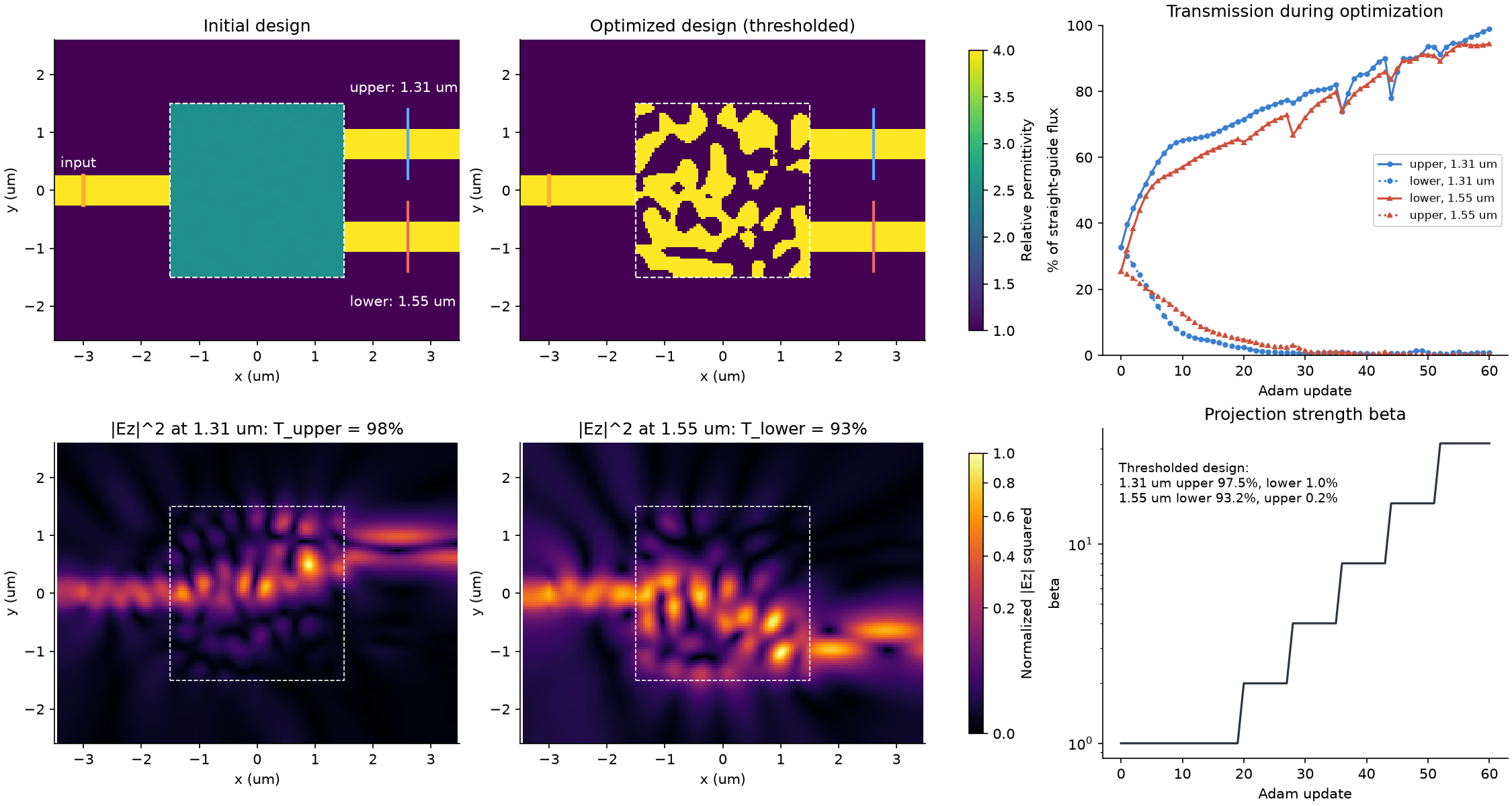
Actual TorchFDTD 1.1.7 run from PyPI: a 3 × 3 µm design region on a 40 nm grid, 5625 density variables with a filter and tanh projection, 60 Adam updates on eight CPU threads (35 min). The thresholded two-level design sends 97.5% of the 1.31 µm light into the upper guide and 93.2% of the 1.55 µm light into the lower guide, with 1.0% and 0.2% in the wrong guide. Transmissions are normalized by a straight guide, so scattering losses count. Conditions and numerical record.
Download optimize.py, then run it with the PyPI package:
pip install torchfdtd matplotlib
python optimize.py --iterations 60 --check-gradient --output results/wavelength-splitter
The core update is below. The linked script supplies the complete project, density parameterization, plotting and result export:
optimizer.zero_grad(set_to_none=True)
epsilon, density = material(theta, project, beta_at(update), background)
t = transmissions(model, epsilon, project, incident)   # [port, wavelength] at 1.31 and 1.55 um
loss = -objective(t)
loss.backward()                         # Discrete adjoint and density/filter gradient
optimizer.step()
The script checks one adjoint derivative against a central finite difference and saves the design arrays, output fluxes, field image and a browser project. You can also download the ready-to-open splitter and load it with torchfdtd serve. Its 64-level CAD approximation fits the default workbench limits and differs by 0.0174% in captured flux from the continuous design. See differentiable planes for the flux API and reversible CPML adjoints for larger designs.
Paper designs: E1, E2, E3
The paper applies tiled 3D full-wave adjoints and differentiable angular-spectrum propagation to three freeform metasurfaces. The repository includes their drivers, configurations, targets, optimized layouts and figure source data.
| Study | Device and target | Re-evaluated objective | Hardware of the reported optimization |
|---|---|---|---|
| E1 | 200 µm lens, nine wavelengths from 420 to 670 nm, common focus at 333.3 µm | J1 = 0.1196 | 8 × H200 |
| E2 | 150 × 150 µm color hologram, 450/540/635 nm, image plane at 300 µm | J2 = 0.6730 | 6 × H200, then 8 × H100 |
| E3 | 100 × 100 µm polarization-switched hologram, CNU/PHY under x/y input at 540 nm, image plane at 200 µm | J3 = 0.8439 | 6 × H200 |
The table reports the saved binary layouts re-evaluated with 3.6 µm tile overlaps. Each study has its own objective definition. The published full-scale runs used the historical solver commit recorded in the reproduction guide.
E1: a nine-wavelength freeform lens
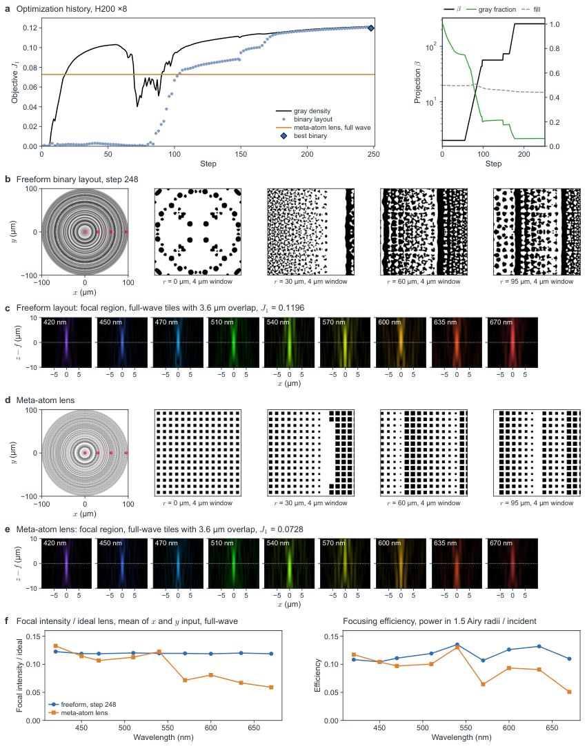
Figure 3 from the authors' public arXiv v3: optimization history, final dielectric pattern and full-wave focal fields of E1. The convergence history uses the 0.9 µm overlaps of the optimization. The optical comparison is re-evaluated with 3.6 µm overlaps.
E2 and E3: color and polarization-switched holograms
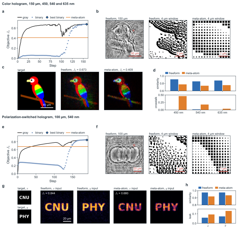
Figure 4 from the authors' public arXiv v3: E2 in the upper panels and E3 in the lower panels. These are the reported full-scale results. Figure provenance · Reproduce or evaluate the saved layouts.
Examples
Each example includes its geometry, run commands and comparison results. AGENTS.md lists a starting example for each common task.
For complete design studies, follow the installed-wheel application workflows: metagrating, finite metalens and photonic integrated circuit, with fixed seeds and acceptance criteria.
| Example | What to explore |
|---|---|
| Microring resonator | A bus-coupled ring, transmission spectra and resonance positions compared with Meep |
| 2D and 3D metalenses | Focusing fields and efficiency compared with Meep |
| Metagrating | Diffraction-order efficiencies compared with Meep and an RCWA reference |
Photonic-crystal waveguide
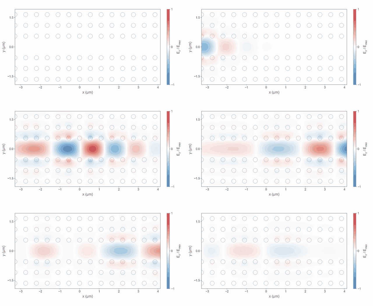
A pulse in a photonic-crystal line-defect waveguide. Actual 2D FDTD, showing instantaneous signed Ez with the dielectric rods outlined in gray. Full-resolution video · Model and recording details.
3D metalens focusing
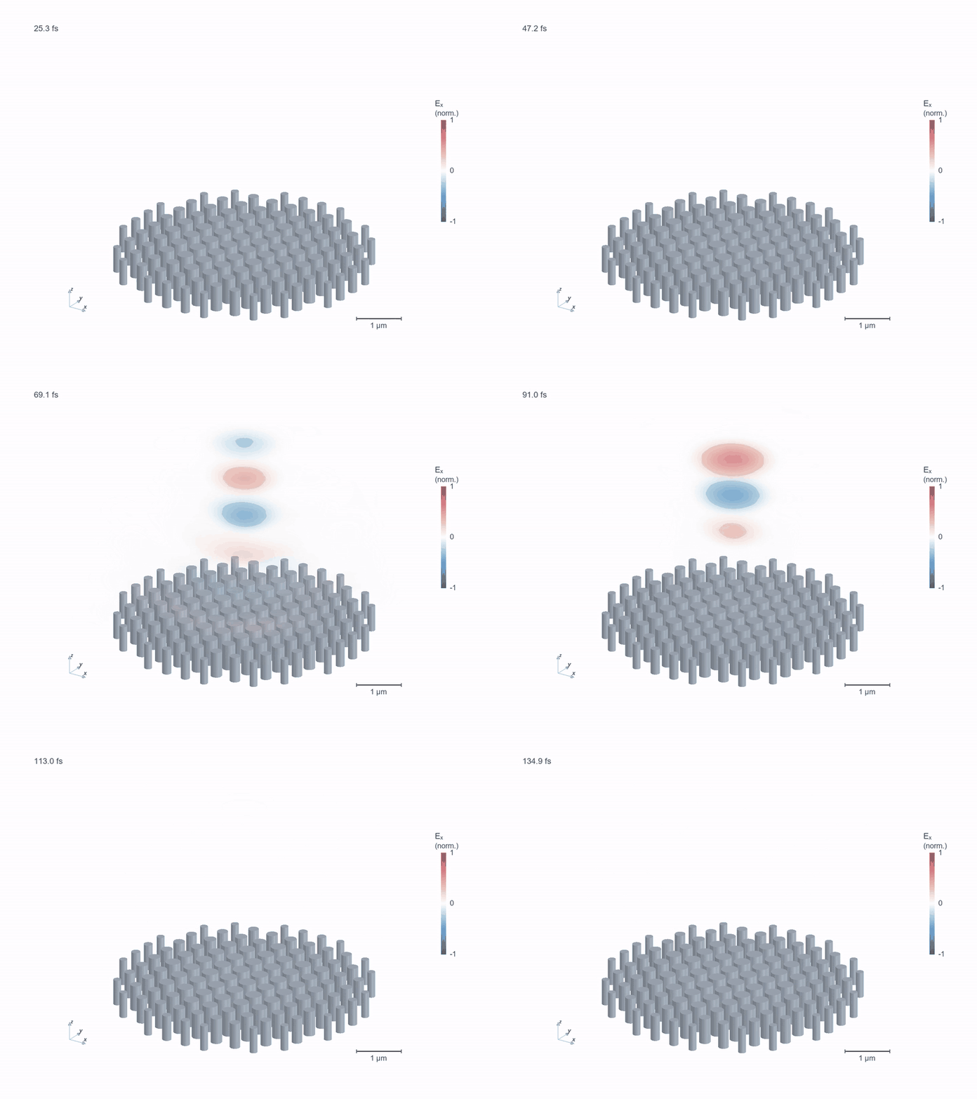
A pulse focusing above a silicon-pillar metalens. Full 3D FDTD, rendered as a translucent volume of instantaneous Ex. Red and blue indicate opposite field signs, with one fixed scale throughout. Full-resolution video · Model and reproduction.
For gradients and optimization, start with differentiable FDTD and shape gradients. For larger studies, see parameter sweeps and tensor batches.
Core features
Materials, boundaries, sources, gradients and memory modes
- Native CUDA engine. Fused Yee and CPML kernels, CUDA Graphs, FP32/FP64, complex Bloch fields, CPU fallback.
- Browser workbench. Objects tree, XY/XZ/YZ and perspective CAD views, materials, simulation region, layout/analysis modes, field viewer, monitor traces, Python export.
- Python first. One
ProjectJSON shared with the browser,BatchRunnerfor independent cases across processes and GPUs with resume,run_tensor_batchfor many structures in one CUDA launch, seeded differential evolution. - Inverse design. Checkpointed and reversible Torch adjoints for dielectric, dispersive (ADE), Bloch, CPML, PEC/PMC, density, polygon/spline shape and source-waveform parameters. Objectives on point signals, plane spectra, N-port S-parameters, far-field and near-zone projections.
- Beyond VRAM. Streamed execution across VRAM, DRAM and NVMe with measured memory reservations, a metadata planner and a crash-resumable journal.
- Physics. 3D and 2D Yee grids, uniform or graded mesh, per-face CPML, periodic/Bloch, PEC/PMC/symmetry, Drude/Lorentz dispersion with passive fitting, anisotropic tensors, subpixel interfaces, point/sheet/plane/one-way/TFSF/mode sources, DFT monitors, mode ports, near-to-far field, diffraction orders.
- Interoperability. GDS import/export with holes, etch layers, sidewall angles and port markers.
Performance and validation
The repository includes analytical tests, convergence and gradient checks, and comparisons with Meep, FDTDX, BeamZ and RCWA. Start with the worked device comparisons or the cross-solver benchmarks. Hardware, precision and problem size are recorded alongside the results.
Detailed benchmarks, execution modes and solver comparisons
How much faster
| Comparison | Setting | Result |
|---|---|---|
| flaport/fdtd on CUDA vs TorchFDTD fused kernels | 64³ and 96³, 800 steps | 16 to 17× and 10 to 12× |
| 16-case parameter sweeps vs flaport/fdtd sequential | 32³ and 64³ | 31 to 44× and 15 to 16× |
| Torch CPU vs GPU, differentiable forward and backward | 128 × 64 × 64, 32 steps | 69× resident, 12× with DRAM streaming |
| CPU worker vs CUDA worker ensemble | 4 × 64³, 800 steps | 40× |
| Meep 1.34 at its fastest rank count (4 MPI ranks on i7-12700) vs TorchFDTD on RTX 3060 | vacuum and sphere, 64³ and 96³, 800 steps, Meep in double precision, TorchFDTD in single | 30 to 36× full solve, 36 to 41× stepping |
| Meep 1.34, 4 MPI ranks on i7-12700 vs TorchFDTD in double precision on an A100 80GB | the same scenes, both solvers in double precision; a data-center GPU against a desktop CPU | 49 to 59× full solve |
| FDTDX 0.6.2 on the same RTX 3060 vs TorchFDTD | vacuum and sphere, 64³ and 96³, 800 steps | 6.4 to 7.3× full solve, 4.4 to 5.7× stepping |
| BeamZ 0.6.2 from PyPI (JAX backend) vs TorchFDTD on the same RTX 5090 | vacuum and sphere, 64³ and 96³, 800 steps | 1.6 to 2.1× full solve, 2.6 to 3.6× stepping |
| FDTDX adjoint (checkpointed, reversible) vs TorchFDTD checkpointed adjoint | 64³, 128 steps, full permittivity gradient, 2 checkpoints, same RTX 3060 | 52× and 2.0× time to gradient, gradients within 1.1e-7 relative |
| Larger than the GPU, capacity run | 2.42 billion cells, 58 GB (54 GiB) of E/H on a 48 GiB GPU, 10 steps plus full material gradient | 2.23 GB peak CUDA memory, 58 min, gradient within 9.1e-8 of the oracle |
| Larger than the GPU, crash and resume | 2.26 billion cells, 54 GB (50.6 GiB) of E/H, same policy | killed after the first backward record, resumed process finishes with 3.03 GB peak CUDA memory and the gradient within 9.1e-8 |
Every row has its conditions, hardware and raw records in docs/MEASUREMENTS.md. The Meep, FDTDX and BeamZ rows come from the same-hardware comparisons in docs/CROSS_SOLVER_COMPARISON.md (BeamZ in section C2, on a rented RTX 5090), which also lists the solver differences behind them; the Meep rows use the 4-rank member of its rank sweep (docs/validation/cross_solver/meep_throughput_ranks4.json), the fastest of 4, 8, 12 and 16 ranks, and the A100 row the double-precision record docs/validation/paper_review/torchfdtd-precision-a100.json. The two beyond-VRAM rows are ten-step capacity gates, not sustained optimizations.
Compared with Meep
Three devices were each set up once from one geometry file and run in TorchFDTD (NVIDIA GeForce RTX 3060, float32, fused CUDA kernels) and in Meep 1.34.0 (CPU, float64, MPI) on the same grid, time step, step count, source, monitors and staircase material sampling, with the agreement criteria declared before the first comparison run. Every number in the table is read from the records in docs/validation/meep_comparison/ by scripts/render_meep_comparison.py; the timing rows are development runs on a shared host (Meep with 4 ranks) until the maintainer's --timing rerun on a quiet host replaces them.
| Device | Cells x steps | Agreement versus its criterion | TorchFDTD GPU stepping (s) | Meep CPU stepping (s), 4 ranks | Ratio |
|---|---|---|---|---|---|
| 2D microring resonator with a bus waveguide (Ez) | 469,500 x 89,219 | resonance wavelengths, max difference 5.6e-05 nm (limit 0.2 nm); 5/5 pass | 31.36 | 217.05 (4 ranks; development run, shared host) | 6.9 |
| 2D silicon ridge metalens (Ez) | 825,600 x 5,200 | focusing efficiency, difference 4.0e-06 (limit 0.01); 4/4 pass | 1.57 | 13.29 (4 ranks; development run, shared host) | 8.5 |
| 3D silicon pillar metalens (Ex) | 3,430,400 x 2,500 | focusing efficiency, difference 2.1e-06 (limit 0.01); 5/5 pass | 6.06 | 128.60 (4 ranks; development run, shared host) | 21.2 |
| 2D silicon metagrating on silica, with an RCWA oracle (Ez) | 18,200 x 12,000 | order efficiencies, max difference 2.0e-04 (limit 0.01); 5/5 pass | 0.26 | 1.49 (4 ranks; development run, shared host) | 5.7 |
Per-example device and fixture tables, all criteria, timing with load notes, figures, run commands and fairness limits: docs/MEEP_COMPARISON.md; the examples live under examples/meep_comparison.
Execution modes
The workbench's FDTD panel has a GPU switch and a Memory selector; /api/validate reports the resolved mode before a run and the results panel reports what ran.
| Mode | When | What it costs | Limits |
|---|---|---|---|
| GPU switch (docs) | A CUDA device is reported; CuPy adds the fused kernels | Nothing beyond the device | Without CuPy the PyTorch kernels run and streamed tiles fall back to the CPU |
| Resident (docs) | The estimate fits 75% of free VRAM and its host arrays 80% of RAM (the whole estimate on CPU); the workbench server also limits it to 8 million cells unless started with --memory-admission |
The fastest path, live frames | The whole grid in one memory |
| Streamed DRAM (docs) | The grid exceeds the device but the conservative reservation fits 80% of available RAM | Slab traffic every temporal block; 5.5 to 11 times the resident time in the records | Forward only, one final snapshot, no dispersive/TFSF/subpixel/PMC scenes |
| Streamed disk (docs) | Explicit opt-in only, never chosen by Auto: the DRAM banks do not fit and scratch space is admitted up to 80% of the free volume | The same slabs through buffered file I/O; 1.9 to 2.4 times the DRAM time in the records | As above, plus a scratch directory to manage |
| Tiled approximate (docs) | A planar device fits neither VRAM nor DRAM; Auto selects it only with the "allow approximate tiling" consent, else the Tiled mode is explicit | Overlapping resident tiles: about 2.5 times the device cells at 1.5 um overlap, longer than the whole device would take | Exact only for an empty region or when every tile holds every scatterer; near-field error of 5 to 12% in the records, read the mismatch indicator; forward only in the browser |
Large devices. Auto keeps a scene resident when it fits, then streams it through DRAM: the streamed X-slab engine stitches its halos exactly, step by step, so a scene that fits either tier gives the resident answer. Disk streaming is exact too but ran 1.9 to 2.4 times slower than DRAM banks in the records, so it is an explicit opt-in that Auto never selects. Tiling is for a device that fits neither, and Auto uses it only with consent; otherwise it refuses and names the options. It is an approximate method whose error decays with the distance to the cuts on a scale of a few micrometres: on a 40 um pillar array cut into 20 um cores, the stitched near field differs from the whole device by 23% at 2 um overlap and 6% at 10 um, by 1.7% more than 10 um from the cuts at that overlap, and the focal intensity by 4% (record). The neighbour mismatch inside the shared overlap is the indicator the workbench shows; it bounds the error (two to four times the stitched error in the records) but does not calibrate it. The tiled adjoint remains a Python API. Beyond the output plane of any of these runs, the workbench's angular-spectrum panel propagates the stored DFT plane through the exterior instead of meshing it: on the recorded metalens the xz section through the focus differs from FDTD through the focus by 1.8% in intensity and took 0.035 s against 60 s (docs/ANGULAR_SPECTRUM.md).
Compared with FDTDX
Ahead: browser CAD, same-GPU structure batches, beyond-VRAM streaming with restart, GDS export and browser import, shape derivatives on top of density parameterization. Equal: nonuniform meshes, dispersive materials, anisotropic materials, boundaries, mode sources and ports, far-field projection, differentiable physics with fixed eigenmodes. Behind: single-problem multi-GPU (experimental slab decomposition, verified bit for bit with CPU, Gloo and single-GPU thread ranks; not yet timed on several GPUs).
Documentation
- Python and batch API, tensor batches, differentiable FDTD, shape gradients
- Streamed execution, planner, restart journal, beyond-VRAM records, propagated case
- Mode ports, far field, GDS, materials, boundaries
- Measurements and feature record, cross-solver comparison with Meep, FDTDX and BeamZ, worked comparisons with Meep
- Security model, compatibility and support policy, changelog, third-party notices and SBOM
Verification
python -m pytest -q
npm run test:ui
The solver benchmark tables use analytical solutions, independently authored CPU/CUDA references, and the open-source solver comparisons linked above. The paper design studies have their own validation and reproduction records in the full-aperture example.
Citing TorchFDTD
If TorchFDTD contributes to published work, please cite the paper and the software on Zenodo. The Zenodo link opens the latest archived release. Citation metadata is available in CITATION.cff, which GitHub offers as "Cite this repository".
The paper is by Hyoseok Park and Yeonsang Park, with Yeonsang Park as the corresponding author.
@misc{park2026torchfdtd,
  author        = {Park, Hyoseok and Park, Yeonsang},
  title         = {Inverse design of large-scale freeform meta-optics by breaking the memory wall of full-wave simulation},
  year          = {2026},
  eprint        = {2609.30039},
  archivePrefix = {arXiv},
  primaryClass  = {physics.optics},
  doi           = {10.48550/arXiv.2609.30039},
  url           = {https://arxiv.org/abs/2609.30039}
}

@software{park_torchfdtd,
  author    = {Park, Hyoseok},
  title     = {{TorchFDTD}},
  year      = {2026},
  publisher = {Zenodo},
  doi       = {10.5281/zenodo.22928834},
  url       = {https://github.com/hyoseokp/TorchFDTD}
}
AI-assisted development
During the development of TorchFDTD, OpenAI GPT-6 Astra and Anthropic Claude Fable 5.1 were used as AI-assisted programming tools to support code prototyping, implementation, refactoring, debugging, test generation, and documentation. The authors defined the numerical formulations, physical assumptions, validation criteria, benchmark protocols, and acceptance thresholds, and reviewed the resulting implementation and numerical results. Solver correctness was independently assessed using analytical reference solutions, numerical convergence studies, finite-difference and automatic-differentiation gradient checks, independently implemented reference calculations, and CPU–GPU parity tests. The authors take full responsibility for the software, methodology, and results reported in this work.
Attribution
flaport/fdtd (MIT) supplies the grid foundation. PyTorch, NumPy, FastAPI, Three.js, Lucide and Vite keep their licenses. Contributions are welcome; back numerical changes with CPU/GPU parity checks and reproducible benchmark conditions. TorchFDTD is not affiliated with Ansys.