
ikeda042/PhenoPixel
ikeda042/PhenoPixel has 169 GitHub stars and 6 forks. GitHot measured -7 stars in 24 hours. Last checked 2026-11-20 08:12 UTC. Last push 2026-11-19.
What you can do
- ND2 management - Upload, list, inspect metadata, download, delete, and parse .nd2 files.
- Cell extraction - Generate cropped cell images, contours, preview frames, and SQLite databases.
- Annotation - Review auto-detected cells and relabel single cells or debris in bulk.
- Cell viewer - Inspect phase, fluorescence, overlays, replot views, fluorescent spots, heatmaps, map views, distributions, and raw images per cell.
Gemessener Sternzuwachs
- in 24h
- -7
- in 7 days
- Verlauf wird gesammelt
- in 15 days
- Verlauf wird gesammelt
- in 1 month
- Verlauf wird gesammelt
Nettoänderungen in überlappenden Zeiträumen, keine Tagessummen. Fehlende Messwerte bleiben leer. Sterne zeigen Interesse, nicht Qualität.
Über uns
PhenoPixel: A web-based bioimage analysis platform for bacterial single-cell microscopy analytics.
Web und AppsREADME.md
OriginalPhenoPixel
PhenoPixel is a FastAPI + React application for microscopy single-cell extraction, annotation, visualization, and batch phenotype analysis. It is designed around ND2 microscopy workflows: upload an ND2 file, extract cell contours, clean labels, inspect individual cells, and export population-level shape and fluorescence descriptors.
The montage below shows a label-1 cell population from microscope_data.db.
The overlay renders fluo1 as magenta and fluo2 as green without scale bars,
with display intensity balanced per cell while avoiding saturation.


Key Features
| Area | What PhenoPixel provides |
|---|---|
| ND2 management | Upload, list, inspect metadata, download, delete, and parse .nd2 files. |
| Cell extraction | Generate cropped cell images, contours, preview frames, and SQLite databases. |
| Annotation | Review auto-detected cells and relabel single cells or debris in bulk. |
| Cell viewer | Inspect phase, fluorescence, overlays, replot views, fluorescent spots, heatmaps, map views, distributions, and raw images per cell. |
| Bulk analysis | Export and visualize cell length, area, fluorescence intensity summaries, heatmap vectors, contours, Map256 strips, raw intensities, and JSON/CSV data. |
| Research reporting | Keep database files, exports, screenshots, and method formulas close to the analysis code for reproducible reporting. |
Requirements
| Component | Notes |
|---|---|
| Python | Local launch examples use python3.14; the Docker backend image uses Python 3.11. |
| Node.js / npm | Required for the React frontend, Docusaurus docs build, and Storybook screenshots. Dependency versions are locked in frontend/package-lock.json. |
| SQLite | Used for extracted cell databases through SQLAlchemy. |
| OpenCV system libraries | Local installs use opencv-python; Docker also installs libgl1 and libglib2.0-0. |
Quick Start
Run the backend and frontend from the repository root in separate terminals.
The local quick-start path uses python3.14; the Docker backend image uses
Python 3.11.
Backend
python3.14 -m venv venv
source ./venv/bin/activate
cd backend
pip install -r requirements.txt
python main.py
Frontend
cd frontend
npm install
npm run dev
If npm reports peer dependency conflicts around Vite and Storybook, use:
npm install --legacy-peer-deps
Local URLs
| Service | URL |
|---|---|
| Backend | http://localhost:3000 |
| Frontend dev server | http://localhost:3001 |
| API base | http://localhost:3000/api/v1 |
| Swagger UI | http://localhost:3000/api/v1/docs |
| OpenAPI JSON | http://localhost:3000/api/v1/openapi.json |
| Health check | http://localhost:3000/api/v1/health |
Input Data
| Item | Notes |
|---|---|
| Primary input | .nd2 files. Upload through the UI or place them under backend/app/nd2files/. |
| Filename rules | Only .nd2 is accepted; path components are stripped and dots in stems are normalized during processing. |
| Channel/layer modes | single, dual, dual(reversed), triple, and quad are supported by the extraction UI/API. |
| Metadata | ND2 metadata can be viewed from the ND2 Manager. Channel count may be inferred when the metadata exposes it. |
| Time/Z data | The parser can expose ND2 frame metadata, but cell extraction expects the selected layer mode to match the frame/channel organization. Validate previews before running large jobs. |
Workflow
1. ND2 Manager
Manage ND2 files: upload datasets, inspect metadata, delete old files, and open a selected ND2 file in Cell Extraction.

2. Cell Extraction
Choose the layer mode, objective scale, Canny threshold (param1), crop size,
and Auto Annotation setting, then start extraction. The backend creates contour
previews and one or more SQLite databases for downstream analysis.

When extraction finishes, review the preview frames. If contours are poor, adjust parameters and re-extract.


3. Database Manager
Cell databases generated by extraction can be uploaded, downloaded, renamed, deleted, and opened for cell-level review.


The cell viewer function panel provides these modes:
| Mode | Description |
|---|---|
Contour |
Show extracted contour coordinates. |
Replot |
Replot a cell in its aligned coordinate system. |
e-means (spatial) |
Cluster intracellular pixel coordinates into a specified number of spatial groups. |
e-means spots |
Detect compact fluorescent spots with e-means initialization and local Gaussian fitting. |
Overlay |
Overlay the contour on the default cell image. |
Overlay Raw |
Overlay fluorescence without contour masking on the raw view. |
Overlay Fluo |
Compose fluorescence channels with selectable colors. |
Heatmap |
Visualize centerline-projected fluorescence intensity. |
Map 256 |
Render a 256-level mapped fluorescence view. |
Map Raw |
Render the mapped view at native pixel scale. |
Distribution |
Plot the intensity distribution for the selected cell/channel. |

Overlay Raw places fluorescence-channel signal on top of the PH image, making
it possible to check fluorescence localization against the original cell
morphology.

Overlay Fluo shows the fluorescence channels as an overlay without the PH
background, which is useful for inspecting signal overlap and channel-specific
patterns.

Heatmap projects fluorescence intensity along the selected cell's long axis.
The target fluorescence channel can be selected before plotting, so the same
cell can be compared across channels.

Map 256 renders fluorescence information as a 256-level intensity map. This
view preserves the spatial pattern inside each cell and is useful for examining
subcellular localization, such as Nucleoid positioning.

The same Map256 representation can also be used at population scale. The
example below arranges Map256 views from the Label 1 population in
microscope_data.db, summarizing Nucleoid localization across the selected cell
group.

Distribution shows a histogram of intracellular fluorescence intensities for
the selected cell/channel.

e-means spots: fluorescent spot detection
e-means spots locates compact, approximately round fluorescence peaks inside
the selected cell. Open the cell's Function Panel, select Draw mode →
e-means spots, leave tuning on Auto, choose a fluorescence channel, and press Calc. The maximum spot count is
fixed at 10. Auto selects the width range and
acceptance thresholds for each cell; no manual σ or SNR input is required.
The selected values appear in the result image. Choose Manual to override
the width range and minimum SNR.
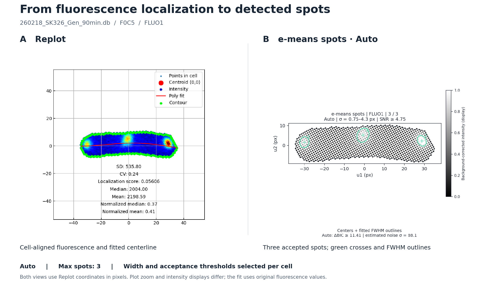
This example uses F0C5 from 260218_SK326_Gen_90min.db, with FLUO1 in
both panels. Auto with a maximum of 3 detects 3 spots, using a width
range of approximately 0.75–4.30 px, Min SNR = 4.75, and ΔBIC ≥ 11.41.
The left panel is
the Replot image (polynomial degree 4, mesh disabled); the right panel is the
e-means spots result. Green crosses mark fitted centers, and green ellipses
show the fitted full width at half maximum (FWHM). Both panels use the same
cell-aligned coordinates in pixels, with different plot zoom and intensity
displays. Open this cell locally.
| Control | Default | Meaning |
|---|---|---|
| Channel | FLUO1 |
Fluorescence image to analyze; FLUO2 is also supported when available. |
| Tuning | Auto |
Estimate the width range, minimum SNR, and BIC requirement for each cell. Manual exposes width and SNR inputs. |
| Max spots | 10 (fixed) |
Upper limit on the number of accepted spots. It does not force the detector to find this many spots. |
| Min σ / Max σ (Manual) | 1 / 4 px |
Allowed Gaussian width along each fitted principal axis. Set 0.5 ≤ Min σ < Max σ ≤ 10. FWHM is approximately 2.355σ. |
| Min SNR (Manual) | 4 |
Minimum fitted peak amplitude above the local background, divided by the estimated noise standard deviation. Allowed range: 2–30. |
For example, Min SNR = 4 requires a fitted peak amplitude at least four times the estimated noise level. Increasing it favors clearer peaks but may miss dim spots; decreasing it admits weaker peaks and can admit more noise. Width, roundness, and model-fit criteria must also pass. Zero detected spots is a valid result. If more candidates pass than the maximum allows, the detector retains those with the largest fitted amplitudes after removing nearby duplicates. Press Calc again after changing settings or cells.
The spot image displays background-corrected intensity scaled to 0–1 using the cell's 99.5th percentile and clipped for display. The fit uses the original fluorescence values; display Gain and this clipping do not affect detection. The color scale therefore does not compare absolute brightness across cells. See the mathematical model and acceptance criteria below.
4. Annotation
Auto-detected contours may include debris or merged cells. Use Annotation to
move cells between N/A and analysis labels such as Label 1. Click cells
individually or use Shift-drag to select multiple cells before applying a label.


5. Bulk Engine
After annotation, use Bulk Engine to run population-level analysis on a selected label. Return to Annotation if non-single cells remain in the selected group.


Bulk Engine modes:
| Mode | Description |
|---|---|
Phenotype map |
Compare eight fluorescence localization descriptors within/across databases using one shared channel and background correction, DB-colored scatter plots, cumulative distributions, quartile summaries, linked images and CSV/JSON exports. |
GFP spot localization |
Normalize detected foci by contour-derived centerline length and local width; compare point clouds, position frequencies and per-cell patterns. Auto detection, at most 10 spots per cell; CSV and SVG exports. |
Cell length |
Measure cell length in pixels from contour geometry. |
Cell width |
Export mean and median full-width estimates in pixels. |
Cell area |
Export cell area in pixels squared. |
Normalized median |
Compute cellwise median intensity after max normalization. |
FITC aggregation ratio |
Report the fraction of cells below the configured normalized-median threshold. |
Entropy |
Quantify fluorescence distribution with entropy / sparsity-style metrics. |
Heatmap |
Generate centerline heatmap vectors and absolute/relative heatmap plots. |
Contours |
Visualize aligned contours and export transformed contour coordinates. |
Map256 |
Render population-level Map256 strips or contour maps. |
Raw data |
Export raw pixel intensities inside each contour. |
GFP spot localization uses cell geometry to compare foci independently of GFP brightness.
The example below shows the first 40 label-1 cells from 260218_SK326_Gen_90min.db
(FLUO1): 77 detected spots, displayed by nearest-pole distance and absolute transverse position.
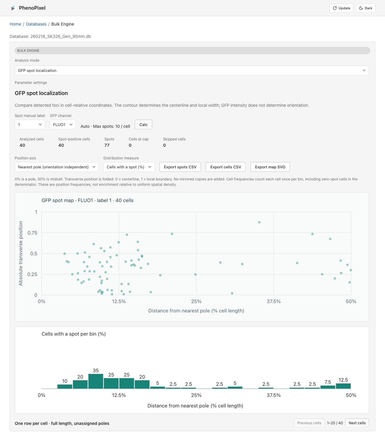
JSON and CSV exports are available for downstream analysis.

For example, Heatmap aggregates and visualizes fluorescence localization for
all cells in the selected label.

Contours mode focuses on contour geometry only. It exports aligned contour
coordinates as JSON or CSV, making it easier to prototype and validate
algorithms that use cell outline information without carrying fluorescence
images or raw intensity data through the analysis pipeline.

Output Data
| Output | Location / format |
|---|---|
| Uploaded ND2 files | backend/app/nd2files/ |
| Cell databases | backend/app/databases/<nd2_stem>.db |
| Extracted contour previews | backend/app/extracted_data/<nd2_stem>/<frame>.png |
| Cell table | SQLite table cells, including cell_id, manual_label, perimeter, area, img_ph, img_fluo1, img_fluo2, contour, center coordinates, objective, and pixel size. |
| Bulk exports | JSON/CSV/PNG responses from Bulk Engine endpoints or browser downloads. |
| Frontend production build | frontend/dist/; the backend serves this folder when it exists. |
Default Parameters
| Parameter | Default / current behavior |
|---|---|
Extraction threshold param1 |
130 |
| Cell crop size | 200 px |
| Default layer mode | dual in the UI |
| Auto Annotation | On by default in the UI |
| Auto Annotation width screen | second PCA variance lambda_2 <= 120 |
| Auto Annotation convexity screen | hull_perimeter / perimeter > 0.85 |
| Extraction concurrency | CELLEXTRACTION_MAX_CONCURRENCY, default 2 |
| Objective presets | 100x = 0.065 um/px, 60x = 0.108 um/px |
| Heatmap vector bins | 35 |
| Centerline polynomial degree | 4 unless a request overrides it |
| FITC aggregation cutoff | 0.7414 |
Methods
The quantitative routines in PhenoPixel follow a common single-cell analysis pipeline: detect a contour from the phase-contrast image, re-parameterize the cell in its intrinsic coordinate system, and compute shape or fluorescence descriptors that are directly comparable across cells. Let $C = {(x_i, y_i)}_{i=1}^n$ be the contour points of one cell and let $\Omega_C$ be the set of pixels inside that contour.
Auto Annotation Model
When Auto Annotation is On, an additional post-processing step runs after
extraction to automatically separate single-cell candidates from debris and
merged cells. The default backend path loads a bundled supervised model from
backend/autoannotation/artifacts/autoannotator.pkl and assigns Label 1 when
the predicted probability is above the trained threshold; otherwise it assigns
N/A.
The model was trained from the bundled reference SQLite dataset
backend/autoannotation/testdata/autoannotation_testdata.db (520 labeled cells:
300 label 1, 220 N/A). The dataset is a single merged DB built from
microscope_data.db and test_database (1).db, with source_db and
source_cell_id provenance columns. Training compares a small set of
dependency-light classifiers and selects the best 5-fold stratified
cross-validation result. The bundled model is an ensemble of weighted
k-nearest neighbors and L2-regularized logistic regression using 96 features
from:
- contour geometry: area, perimeter, circularity, convexity, solidity, bounding box extent, PCA axis variances, eccentricity, and Hu moments.
- cropped images: PH/Fluo contour-inside and outside-ring intensity quantiles, contrast, gradient, and edge-density descriptors.
The selected model achieved F1 0.9608, accuracy 0.9538, precision 0.9423,
and recall 0.9800 in 5-fold CV. The previous contour-only rule remains as a
safe fallback when the model file cannot be loaded or feature extraction fails.
Set PHENOPIXEL_AUTOANNOTATION_MODEL=/path/to/autoannotator.pkl to use a
different trained model.
The fallback contour screen computes two geometric scores. After a contour
$C = {(x_i, y_i)}_{i=1}^N$ is extracted, the backend computes the smaller PCA
axis variance and convexity, and assigns Label 1 only when both pass their
thresholds. First, it measures how thick the contour is in the direction
orthogonal to the major axis. Let
$$ \Sigma_C = \frac{1}{N-1} \sum_{i=1}^{N} (\mathbf{p}_i - \bar{\mathbf{p}}) (\mathbf{p}_i - \bar{\mathbf{p}})^{\mathsf{T}}, \qquad \mathbf{p}_i = (x_i, y_i)^{\mathsf{T}}. $$
If the eigenvalues of $\Sigma_C$ are $\lambda_1 \ge \lambda_2$, Auto Annotation uses the smaller one, $\lambda_2$, as a width / lateral-spread proxy and accepts only contours satisfying
$$ \lambda_2 \le 120. $$
Second, it measures contour convexity from perimeter ratios. If $P(C)$ is the contour perimeter and $P(\mathrm{Hull}(C))$ is the perimeter of its convex hull, the code defines
$$ \kappa(C) = \frac{P(\mathrm{Hull}(C))}{P(C)}. $$
Because irregular debris or merged objects tend to have a perimeter much longer than their convex hull, they produce smaller $\kappa$. The contour is accepted only when
$$ \kappa(C) > 0.85. $$
The final Auto Annotation score can be written as
$$ s(C) = \mathbf{1}[\lambda_2 \le 120] , \mathbf{1}[\kappa(C) > 0.85]. $$
The fallback assigns Label 1 when $s(C) = 1$ and N/A otherwise. In other
words, it keeps contours that are both laterally compact and close to convex.
1. Contour Extraction, Principal Axis, and Basis Transform
Contours are extracted from phase-contrast images with a Canny-based pipeline. The major elongation axis is estimated from the covariance of contour coordinates,
$$ \Sigma = \begin{pmatrix} \mathrm{Var}[X_1] & \mathrm{Cov}[X_1, X_2] \ \mathrm{Cov}[X_1, X_2] & \mathrm{Var}[X_2] \end{pmatrix}, $$
and the principal direction is the solution of
$$ \mathbf{w}^* = \underset{|\mathbf{w}| = 1}{\mathrm{arg,max}} \mathbf{w}^{\mathsf{T}} \Sigma \mathbf{w}, \qquad \Sigma \mathbf{w} = \lambda \mathbf{w}. $$
If $Q = (\mathbf{v}_1\ \mathbf{v}_2)$ is the orthonormal eigenvector basis, coordinates are transformed to the cell-aligned frame by
$$ \mathbf{u} = Q^{\mathsf{T}} \mathbf{x}, \qquad \mathbf{x} = Q \mathbf{u}. $$
This removes arbitrary image rotation and makes bent or filamentous cells easier to model analytically.
Because $Q$ is orthonormal, this basis conversion also preserves Euclidean length. For any vector $\mathbf{x}$ and its transformed coordinate $\mathbf{u} = Q^{\mathsf{T}}\mathbf{x}$,
$$ |\mathbf{u}|^2 = \mathbf{u}^{\mathsf{T}}\mathbf{u} = (Q^{\mathsf{T}}\mathbf{x})^{\mathsf{T}} (Q^{\mathsf{T}}\mathbf{x}) = \mathbf{x}^{\mathsf{T}} Q Q^{\mathsf{T}} \mathbf{x} = \mathbf{x}^{\mathsf{T}} \mathbf{x} = |\mathbf{x}|^2, $$
since $Q^{\mathsf{T}}Q = QQ^{\mathsf{T}} = I$. Therefore distances measured before and after the basis transform are identical.
2. Centerline Fitting and Cell Length
In the aligned frame, the cell centerline is approximated by a $k$-th order polynomial
$$ \hat{f}(u_1) = \theta^{\mathsf{T}} \phi(u_1), \qquad \theta = (W^{\mathsf{T}} W)^{-1} W^{\mathsf{T}} f. $$
For a curved cell, the thesis formulation defines cell length as the arc length between the two contour-centerline intersection points:
$$ L = \int_{u_{1,a}}^{u_{1,b}} \sqrt{1 + (\frac{d\hat{f}}{du_1})^2},du_1. $$

In the current backend implementation, Cell length is returned as the PCA
major-axis extent of pixels inside the contour, in pixels:
$$ L_{\mathrm{px}} \approx \max_i \pi_i - \min_i \pi_i. $$
3. Cell Area and Raw Pixel Export
Cell area is the area enclosed by the contour,
$$ A(C) = \iint_{\Omega_C} 1,dA, $$
which is stored during extraction and reported by Cell area. Raw data
exports the unaggregated intensity set
$$ { I(p) \mid p \in \Omega_C } $$
for the selected channel.
4. Fluorescence Vectorization Along the Centerline
For each intracellular pixel $(p_i, q_i)$ with intensity $G(p_i, q_i)$, the nearest point on the fitted centerline is found by
$$ u_{1,i}^* = \underset{u_1 \in [u_{1,a}, u_{1,b}]}{\mathrm{arg,min}} [(u_1 - p_i)^2 + (\hat{f}(u_1) - q_i)^2]. $$
This position is converted to arc length,
$$ \ell(u_1) = \int_{u_{1,a}}^{u_1} \sqrt{1 + (\hat{f}'(t))^2},dt, \qquad \ell_i^* = \ell(u_{1,i}^*). $$
To obtain a fixed-dimensional descriptor, the arc-length interval $[0, L]$ is divided into $n$ bins and max-pooled:
$$ g_j = \max { G(p_i, q_i) \mid \ell_i^* \in I_j }. $$
If no projected pixel falls into $I_j$, we set $g_j = 0$. The resulting fixed-length localization vector is
$$ \mathbf{g} = (g_1, \dots, g_n)^{\mathsf{T}}. $$
The current implementation uses $n = 35$ and a default polynomial degree of
$k = 4$. Heatmap visualizes these peak vectors either in absolute-length
coordinates or in relative-position coordinates.

5. Map256 Spatial Intensity Mapping
Map 256 keeps more spatial information than the 35-bin heatmap vector. It uses
the same cell-aligned coordinate system and polynomial centerline, but instead
of reducing each longitudinal bin to a single peak value, it remaps every
intracellular fluorescence pixel onto a two-dimensional long-axis / lateral-axis
image.
Before mapping, the selected fluorescence image is converted to grayscale and background-subtracted with a morphological opening:
$$ I_{\mathrm{bg}} = I - \mathrm{open}_{21 \times 21}(I). $$
For each pixel $\mathbf{u}i = (u{1,i}, u_{2,i})$ inside the contour, the nearest point on the fitted centerline $\hat{f}$ is found as
$$ t_i^{\star} = \underset{t \in [u_{1,a}, u_{1,b}]}{\mathrm{arg,min}} \left[(t - u_{1,i})^2 + (\hat{f}(t) - u_{2,i})^2\right]. $$
The projected long-axis coordinate is the centerline arc length,
$$ p_i = \int_{u_{1,a}}^{t_i^{\star}} \sqrt{1 + (\hat{f}'(t))^2},dt, $$
and the signed lateral coordinate is
$$ d_i = \mathrm{sign}(u_{2,i} - \hat{f}(t_i^{\star})) \sqrt{(t_i^{\star} - u_{1,i})^2 + (\hat{f}(t_i^{\star}) - u_{2,i})^2}. $$
These coordinates define a high-resolution map $H \in \mathbb{R}^{h \times w}$, where
$$ w = \lceil \max_i p_i - \min_i p_i \rceil + 1, \qquad h = \lceil \max_i d_i - \min_i d_i \rceil + 1. $$
Each intracellular pixel is assigned to integer map coordinates
$$ x_i = \lfloor p_i - \min_j p_j \rfloor, \qquad y_i = \lfloor d_i - \min_j d_j \rfloor, $$
and intensities are max-pooled into the mapped image:
$$ H(y_i, x_i) = \max\left(H(y_i, x_i), I_{\mathrm{bg}}(\mathbf{u}_i)\right). $$
The implementation also writes the same value to the four direct neighbors $(y_i \pm 1, x_i)$ and $(y_i, x_i \pm 1)$ when they are inside the map. This small local expansion reduces holes caused by integer projection.
For Map 256, the high-resolution map is resized by nearest-neighbor
interpolation to a fixed display size:
$$ M_c \in \mathbb{R}^{256 \times 1024} = \mathrm{resize}_{\mathrm{nearest}}(H_c). $$
The display image is then converted to 8-bit intensity,
$$ \tilde{M}_c = 255 \cdot \frac{M_c - \min(M_c)} {\max(M_c) - \min(M_c)}, $$
with a zero image used when the map has no intensity range. Map Raw keeps the
native high-resolution map before the fixed-size resize. The Jet view applies a
pseudocolor map to the same normalized intensity image.
For population-level Map256 contour plots, the backend first builds one map per cell. To make the population summary less sensitive to arbitrary left/right or top/bottom orientation, each cell contributes four symmetric variants: the original map, left-right flip, top-bottom flip, and both flips. The population mean map is
$$ \bar{M} = \frac{1}{4N} \sum_{c=1}^{N} \left[ M_c + F_x(M_c) + F_y(M_c) + F_y(F_x(M_c)) \right], $$
where $F_x$ and $F_y$ denote horizontal and vertical flips. In relative mode,
each cell map is normalized before averaging; in absolute mode, the
background-subtracted raw intensities are averaged. This makes Map256 useful for
summarizing subcellular localization patterns, such as Nucleoid positioning,
across a labeled cell population. The square montage below was generated from
all Label 1 cells in the current microscope_data.db.
6. Normalized Median and Aggregation-Style Scores
For any selected channel, intensities inside a cell are normalized by the cellwise maximum,
$$ \tilde{I}i = \frac{I_i}{\max{p \in \Omega_C} I(p)}, \qquad m(C) = \mathrm{median}(\tilde{I}_i). $$
This scalar is reported by Normalized median. A population-level aggregation
score can then be written as
$$ R(\tau) = \frac{1}{N} \sum_{c=1}^{N} \mathbf{1}[m(C_c) < \tau]. $$
The current FITC aggregation ratio plot uses this form with a default cutoff
$\tau = 0.7414$. In the thesis experiments, the same normalized-median idea was
also used for IbpA-GFP and TorA-GFP abnormal-localization calls, with an example
threshold of $m \le 0.6$ for those datasets.
7. Thesis-Specific Phenotype Calls
For HU-GFP compaction, a 35-bin peak vector is first computed and summarized as
$$ s(C) = \sum_{j=1}^{35} g_j. $$
Using the control population, the abnormality threshold is defined by the 5th percentile,
$$ \tau_{\mathrm{HU}} = Q_{0.05}({ s(C_c^{\mathrm{ctrl}}) }), $$
and the HU aggregation ratio is the fraction of cells with $s(C) < \tau_{\mathrm{HU}}$.
For PI permeability, the mean intracellular PI intensity is
$$ \mu(C) = \frac{1}{|\Omega_C|} \sum_{p \in \Omega_C} I_{\mathrm{PI}}(p), $$
with a control-derived positivity threshold
$$ \tau_{\mathrm{PI}} = Q_{0.95}({ \mu(C_c^{\mathrm{ctrl}}) }). $$
The PI-positive fraction is then the proportion of cells satisfying $\mu(C) > \tau_{\mathrm{PI}}$.
8. e-means Spots Model
The detector combines three steps:
- Estimate background by morphological opening, then find local maxima of the scale-normalized Laplacian of Gaussian (LoG) response over the selected spot-width range. Candidate centers must lie inside the cell contour.
- Sample nearby Replot coordinates with probability proportional to positive, background-corrected intensity. Run e-means on these samples to initialize centers (5 epochs, fixed seed 1234). This sampling makes bright pixels more influential during initialization.
- Fit each candidate's local, original fluorescence values to an elliptical Gaussian plus a background plane:
$$ \widehat I(\mathbf r) = b_0 + \mathbf g^{\mathsf T}\mathbf r
- A\exp!\left[-\frac12(\mathbf r-\boldsymbol\mu)^{\mathsf T} \Sigma^{-1}(\mathbf r-\boldsymbol\mu)\right]. $$
Here $\boldsymbol\mu$ is the spot center, $A$ is its peak amplitude above the background plane, and the square roots of the eigenvalues of $\Sigma$ are its two Gaussian widths, $\sigma_1$ and $\sigma_2$. Fitted centers and shapes are transformed back into the Replot coordinate system for display. These coordinates remain in pixels; they are not normalized to 0–1.
A candidate is accepted only if the fit converges, its center remains inside the contour, both widths fall within the selected range, and the following conditions hold:
$$ \frac{\max(\sigma_1,\sigma_2)}{\min(\sigma_1,\sigma_2)}\leq 1.6, \qquad \mathrm{SNR}=\frac{A}{\widehat\sigma_{\mathrm{noise}}} \geq \mathrm{Min\ SNR}. $$
The noise estimate is the larger of two robust estimates: one from adjacent intracellular pixel differences and one from the local fit residuals, both based on median absolute deviation (MAD). The spot model must also improve on a background-plane-only model by at least $T_{\mathrm{BIC}}$ BIC units (10 in Manual; selected per cell in Auto):
$$ \Delta\mathrm{BIC} = n\log!\left(\frac{\mathrm{RSS}{\mathrm{background}}} {\mathrm{RSS}{\mathrm{spot}}}\right)-6\log n \geq T_{\mathrm{BIC}}. $$
Both residual sums of squares use the same $n$ local pixels. The background model has 3 parameters and the spot model has 9, so the penalty accounts for 6 additional parameters. e-means supplies initial centers; the fluorescence fit and acceptance criteria determine the final detections.
Automatic acceptance settings
Auto recomputes settings from the current cell at each calculation. It uses the largest distance $R$ from an intracellular pixel to the outside of the contour, measured with a Euclidean distance transform, to set the width range:
$$ \sigma_{\min}=0.75\ \mathrm{px},\qquad \sigma_{\max}=\mathrm{clip}(R/2,,1.5,,10)\ \mathrm{px}. $$
This is a compact-spot prior relative to cell thickness. Widths are still estimated individually by each Gaussian fit. For $N$ intracellular pixels and $L=9$ search scales, the SNR reference is
$$ T_{\mathrm{SNR}}=\max!\left(3,\Phi^{-1}!\left(1-\frac{0.01}{NL}\right)\right), \qquad T_{\mathrm{BIC}}=\max!\left(10,2\log\frac{\max(1,M)}{0.01}\right), $$
where $\Phi$ is the standard normal CDF and $M$ is the number of LoG proposals retained for fitting (up to 64). Larger searches require stronger evidence. The absolute amplitude cutoff also follows the robust noise estimate, which is recomputed from the cell and each fit's residuals. The proposal limit is independent of the fixed Max spots limit, which only caps the accepted results in Auto. Thresholds are never lowered just to fill the requested count.
Auto reduces user inputs; it is not parameter-free. The compact-width prior,
axis-ratio limit of 1.6, and internal reference budget of 0.01 remain fixed.
The Gaussian-tail and BIC rules are application heuristics, not a guarantee
of a 1% false-positive rate, especially for correlated or non-Gaussian noise.
The API enables Auto with auto_tune=true on get-cell-e-means-spots; omitted
or false retains Manual behavior for existing API clients.
These are approximate Gaussian-noise/model-selection criteria, not calibrated
detection probabilities or significance levels. Candidates are fitted
individually, so closely overlapping spots may be missed or merged; diffuse
or elongated signals can fail the width or roundness criteria. Implementation:
spot_detection.py.
Research Use / Citation
This repository is maintained to support reproducible reporting in research papers. If you cite this software in a manuscript, include:
- Software name: PhenoPixel
- Author: Yunosuke Ikeda
- Contact: [email protected]
- Repository URL: this repository URL
- Version evidence: Git commit hash used in the analysis
- Access date: date you accessed the repository
Recommended citation:
Ikeda, Y. PhenoPixel: microscopy single-cell extraction and batch phenotype analysis software.
GitHub repository. URL: <repository-url> (accessed <YYYY-MM-DD>), commit <commit-hash>.
For reproducibility, report OS/Python/Node versions, dependency snapshots, ND2 metadata or acquisition conditions, extraction parameters, labeling criteria, Bulk Engine modes, thresholds, export settings, and the exact commit hash.
Cellpose-SAM
The Mother Machine workflow uses Cellpose 4.2.1.1 with the updated
cpsam_v2 Cellpose-SAM model for cell segmentation. Analyses that use this
workflow should also cite the Cellpose-SAM paper:
Pachitariu, M., Rariden, M., & Stringer, C. (2025). Cellpose-SAM: superhuman generalization for cellular segmentation. bioRxiv, 2025.04.28.651001. https://doi.org/10.1101/2025.04.28.651001
Software resources:
- Cellpose package: https://pypi.org/project/cellpose/
- Cellpose source code: https://github.com/MouseLand/cellpose
- Cellpose documentation: https://cellpose.readthedocs.io/
Development And Quality Checks
Backend checks:
source ./venv/bin/activate
PYTHONPATH=backend python -m unittest discover backend/tests
Frontend checks:
cd frontend
npm run build
npm run lint
Screenshot/storybook assets:
./docs/make_screenshots.sh
Production Build
Build the frontend before serving the app from the backend:
cd frontend
npm install --legacy-peer-deps
npm run build
cd ../backend
source ../venv/bin/activate
python main.py
When frontend/dist/index.html exists, backend/main.py serves the SPA and
static assets alongside the /api/v1 API.
Docker Deploy (Traefik)
docker/compose.yaml starts Traefik and the backend container. The current
compose file exposes the backend under /api/v1/ and mounts persistent backend
data directories.
Create backend/.env first:
cp backend/.env.template backend/.env
Environment variables used by local/Docker deployment:
| Variable | Used by | Meaning |
|---|---|---|
SLACK_WEHBOOK_URL |
Backend | Optional Slack webhook URL for job notifications. The variable name intentionally matches the current code/template spelling. |
BASE_PATH |
Backend | Optional frontend base URL used in Slack notification links. |
CELLEXTRACTION_MAX_CONCURRENCY |
Backend | Optional extraction job concurrency limit; defaults to 2. |
SERVER_HOST |
Docker compose / Traefik | Hostname routed to the backend; compose defaults to localhost when unset. |
TRAEFIK_ACME_EMAIL |
Docker compose / Traefik | Email address for Let's Encrypt certificate registration. |
Start the stack:
cd docker
docker compose -f compose.yaml up -d --build
Traefik uses ports 80 and 443. Access the hostname set in SERVER_HOST;
the API is exposed under /api/v1.
Troubleshooting
| Symptom | What to try |
|---|---|
| Port already in use | Backend defaults to 3000, frontend to 3001, docs dev server to 3002; stop the existing process or change the port. |
eslint: command not found |
Install frontend dependencies with npm install or npm install --legacy-peer-deps. |
| npm peer dependency conflict | Use npm install --legacy-peer-deps, matching docs/make_screenshots.sh. |
| ND2 upload is rejected | Confirm the file extension is .nd2 and the filename does not rely on path components. |
| No contours or poor contours | Check layer mode, param1, crop size, and preview frames before annotating. |
| OpenCV import/runtime errors | Use the project venv and install backend/requirements.txt; Docker also installs libgl1 and libglib2.0-0. |
| SQLite permission errors | Ensure backend/app/databases/, backend/app/extracted_data/, backend/app/nd2files/, and backend/app/tempdata/ are writable. |
Tech Stack
Backend:


- FastAPI, Uvicorn, and Pydantic for the API layer
- SQLAlchemy and SQLite for database access
- NumPy, OpenCV, Pillow, and Matplotlib for image processing and plotting
- FastMCP for repository/context tooling
Frontend:


- React + React Router for the UI
- Vite for dev/build tooling
- Chakra UI and Framer Motion for styling and motion
- Docusaurus docs build under
frontend/docs-site
Docs
License
PhenoPixel is released under the MIT License. See LICENSE for details. Third-party dependencies remain under their respective licenses.